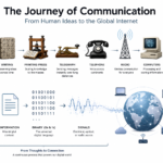
Application:DNS translates names to IPs, DHCP automates IP assignment via the DORA handshake, and HTTP/3 delivers web assets.
Transport:TCP guarantees bit-perfect, ordered delivery via a 3-way handshake, while UDP provides fire-and-forget speed for real-time streaming and gaming.
Internet:IPv4/IPv6 handle logical addressing. Routers deploy BGP path-vector policies to connect independent global networks.
Network Access:Ethernet Frames execute local delivery using hardware MAC addresses. VLANs (802.1Q) segment broadcast domains, and LACP aggregates physical links to scale bandwidth.
2. Problem & Solution Matrix
Network Problem
Root Cause
Technical Solution
Operational Impact
IP Address Exhaustion
32-bit IPv4 design limits
IPv6 Scaling & NAT/PAT
Provides an inexhaustible pool of global IP numbers.
Head-of-Line Blocking
TCP stream-ordering freezes
QUIC Protocol (over UDP)
Single packet drops no longer stall the remaining data queue.
Data Center Bottlenecks
Legacy hierarchical design delays
Spine-and-Leaf Clos
Predictable, non-blocking 2-hop fabric for East-West traffic.
Physical Cable Loops
Redundant path broadcast storms
Spanning Tree (STP)
Blocks loop paths while maintaining active backup links.
Out-of-Order Frames
Multi-cable path propagation variations
LACP Flow Pinning
Hashes metadata to lock specific traffic flows to a single wire.
3. Three Engineering Laws
Switches run blind to IP: Local traffic routes strictly by Layer 2 MAC addresses. Cross-layer translation is managed entirely by ARP (IPv4) and NDP (IPv6).
Bandwidth $\neq$ Latency: Expanding bandwidth widens the data pipe, but latency is a physical constraint bound by the speed of light in fiber glass.
The Web is leaving TCP: Next-gen traffic runs on HTTP/3 over QUIC. By running over UDP, it eliminates handshake delays and prevents session drops when switching networks (e.g., Wi-Fi to cellular).
PREREQUISITE CHECK: If you are skipping straight to protocol logic without mastering how raw electricity is quantized into bits, back up. Revisit the mathematical boundaries of the wire in Volume I: The Architectural Foundations of Information before tracing live packet streams below.
[ Structural Mapping ] ──> Flat definition of the 7 layers without execution context.
[ TechZero Interface ] ──> An active systems schematic tracing how abstract software
                            boundaries map to real-world memory structures and network drivers.
Why This Chapter Matters
In production systems engineering, troubleshooting network failures without a clear reference model leads to a chaotic guessing game. When a microservice fails to connect or a cloud router drops packets, an infrastructure architect must instantly isolate whether the root cause is a physical hardware fault, an optical signal degradation, a routing loop, or a cryptographic handshake mismatch. Reference models provide the technical map required to organize, build, and debug complex distributed applications. This chapter breaks down the OSI and TCP/IP architectural stacks, transforming abstract layer definitions into a practical map for system debugging.
30-Second Smart Summary
Reference models partition the overwhelming complexity of global networking into distinct, manageable operational layers:
The OSI Model provides a 7-layer theoretical blueprint that isolates responsibilities from physical signaling up to human software application logic.
The TCP/IP Model is a compressed, 4-layer production model that directly runs the modern public internet.
Every layer interacts strictly through well-defined Interfaces, treating the data layer immediately above it as a completely opaque payload.
Learning Objectives
Map real-world network operations, hardware components, and software protocols to their exact layers in both the OSI and TCP/IP models.
Contrast the theoretical utility of the OSI framework with the practical, implementation-driven design of the TCP/IP stack.
Analyze the flow of a data unit as it moves down the transmission stack and up the receiving system.
Core Concepts
The Two Frameworks Mapping Matrix
To navigate system architectures, you must maintain an absolute understanding of how the theoretical OSI layers correspond to the practical TCP/IP suite running in production kernels:
OSI Layer
Layer Name
Core Responsibility
Data Unit
Hardware/Software Examples
TCP/IP Equivalent
Layer 7
Application
Human-machine software interaction.
Data
HTTP/3, SSH, SMTP, DNS
Higher Layers
Layer 6
Presentation
Data syntax formatting, translation, and encryption.
Data
TLS, JSON serialization, ASCII
(Combined into
Layer 5
Session
Managing long-term authentication connections.
Data
Sockets API, RPC session trackers
Application)
Layer 4
Transport
End-to-end host communication and data integrity.
Segment / Datagram
TCP, UDP, QUIC
Transport
Layer 3
Network
Logical addressing and cross-network packet routing.
Packet
IP (IPv4/IPv6), BGP, Routers
Internet
Layer 2
Data Link
Local node-to-node framing and physical addressing.
Frame
Ethernet, Wi-Fi, MAC addresses, Switches
Network
Layer 1
Physical
Modulating raw bit arrays onto physical mediums.
Bits
Fiber optics, Cat6 copper, Radio frequencies
Access
Deep Dive: Theoretical Purity vs. Production Reality
==================================================================================
                 THE REFERENCE MODEL EVOLUTIONARY DIVIDE
==================================================================================
  OSI REFERENCE BLUEPRINT (Layer Isolation Focus)
  [App] ──> [Pres] ──> [Sess] ──> [Transport] ──> [Network] ──> [Data Link] ──> [Phys]
  * Status: Highly descriptive academic standard. Complicated to implement cleanly in software.

  TCP/IP INTERNET SUITE (Running Code Optimization)
  =================== [ Application Layer ] =================== (Gutenberg/App Space)
  =================== [ Transport Layer   ] =================== (OS Kernel Space)
  =================== [ Internet Layer    ] =================== (OS Kernel Space)
  =================== [ Network Access    ] =================== (Hardware Driver Space)
  * Status: The functional, lightweight standard running every active node on Earth.
==================================================================================
The OSI Model’s Seven Layers
Developed by the International Organization for Standardization (ISO) in the late 1970s, the Open Systems Interconnection (OSI) model was an academic, highly descriptive framework. Its 7 layers were engineered under a strict architectural rule: each layer must perform a well-defined set of functions, and its boundaries must be isolated from its neighbors to prevent changes in one layer from breaking the others. However, the model proved too heavy for rapid software development. Writing separate applications, session managers, and data formatters created excessive memory allocation checks that severely slowed down early networking kernels.
The TCP/IP Model’s Lean Architecture
While the OSI model was being debated in academic committees, defense and university researchers were building the practical TCP/IP protocol suite on real hardware. The resulting 4-layer model prioritized engineering efficiency, speed, and clean code implementation over theoretical isolation:
Application Layer: Merges the OSI’s Application, Presentation, and Session functions into a unified software layer. Web browsers, database query engines, and API endpoints manage their own sessions, serialize data (e.g., into JSON arrays), and format payloads directly.
Transport Layer: Maps directly to OSI Layer 4. It establishes connection rules between endpoints, handles error checking, and tracks segments.
Internet Layer: Corresponds to OSI Layer 3. It handles logical packet routing across multiple networks using the standard Internet Protocol (IP).
Network Access Layer: Combines OSI Layers 1 and 2. It handles the local physical network interfaces, framing data onto local copper, fiber, or wireless mediums via hardware drivers and network interface cards (NICs).
Engineering Perspective: Navigating Layer Boundaries During Debugging
As an infrastructure engineering professional, reference models serve as a mental flowchart for troubleshooting high-priority system incidents. Consider how an engineer isolates the cause of an application failure:
[ Problem: App cannot write to remote database ]
   │
   ├── Step 1: Run 'ping'. Can packets route to the target IP? ── (Testing the Internet Layer)
   │     └── NO: The problem is a broken routing path or static configuration error. Stop here.
   │
   ├── Step 2: Run 'telnet' on the port. Can a handshake open? ── (Testing the Transport Layer)
   │     └── NO: The server firewall is actively blocking connection blocks. Stop here.
   │
   └── Step 3: Inspect TLS certificates and payload API logs. ──── (Testing the Application Layer)
         └── YES: The network is healthy; the problem is an unhandled code bug or invalid token string.
By working methodically through the network layers from the bottom up, you avoid wasting time debugging application code logic when the actual issue is a bad physical fiber connection or a misconfigured routing table entry.
Real-World Case Study: The Mismatched Layer Configuration Incident
In 2023, a cloud engineering team deployed a multi-tier database cluster across an enterprise hybrid cloud environment. After a mandatory security patch update to the hypervisor host nodes, the database instances began experiencing random connection timeouts and performance drops.
* Symptoms: Low throughput, packet drops during high-volume data synchronization cycles.
* Initial Guess: Software engineers assumed an application-layer database locking bug.
* Actual Root Cause: The hypervisor update had reset the physical NIC interfaces to standard 1500-byte MTU limits, while the cloud overlay network was wrapping data in extra tunnel headers that pushed packet sizes to 1550 bytes, forcing the Data Link/Internet layers to continuously fragment the data streams.
The database application layer was generating payloads perfectly, but the lower layers were choking on the oversized packets. Once the platform engineers identified the layer mismatch, they configured Jumbo Frames (9000-byte MTU) across the network interfaces. This allowed the encapsulated frames to travel smoothly at line rate, immediately resolving the database timeouts and restoring normal operations.
Common Misconceptions
Myth: Modern software operating systems run explicit, independent software modules for each of the seven individual layers outlined in the OSI model.
Reality: The OSI model is a conceptual tool. In modern kernels (like Linux or Windows), the network stack combines these layers into highly optimized, integrated systems spaces—splitting work between user application code, kernel networking loops, and specialized hardware interface controllers (NIC ASICs).
TechZero Insight
When designing high-frequency trading platforms or ultra-low latency microservices, remember that every transition between reference model layers adds processing latency. Passing data from user application space, down through the operating system’s kernel transport memory buffers, and into the physical network interface card adds performance overhead. To bypass this bottleneck, high-performance systems use specialized techniques like Kernel Bypass (DPDK/SR-IOV). This architecture allows application code to write bits directly to the physical network card memory blocks, bypassing the kernel layers entirely to drop connection latency to single-digit microseconds.
Key Takeaways
The OSI model functions as a descriptive, seven-layer structural conceptual framework for network design.
The TCP/IP suite is a practical, implementation-driven four-layer layout that directly powers production systems.
OSI Model: A theoretical seven-layer network reference architecture developed to standardize global communications protocols.
TCP/IP Model: The four-layer protocol suite standard that serves as the baseline architecture for the public internet.
Interface: The structured boundary and rules defining how adjacent layers within a network stack exchange data.
Kernel Bypass: A performance optimization technique that lets applications bypass the operating system’s network stack to write data directly to network hardware.
Suggested Reading
Zimmermann, Hubert, “OSI Reference Model—The ISO Model of Architecture for Open Systems Interconnection”, IEEE Transactions on Communications, 1980.
Comer, Douglas E., Internetworking with TCP/IP, Volume 1: Principles, Protocols, and Architecture, Pearson, 6th Edition, 2013.
References
ISO/IEC 7498-1: Information Technology—Open Systems Interconnection—Basic Reference Model (Official Specifications).
IETF RFC 1122: Requirements for Internet Hosts—Communication Layers (Definitive TCP/IP Model Guidelines).
Review Questions
Explain why the TCP/IP implementation chose to merge the OSI Session, Presentation, and Application layers into a single operational architecture.
Trace the structural path of a data payload as it moves down through the TCP/IP stack on a transmission host, identifying the specific data units generated at each layer boundary.
Chapter 2. The Data Link Layer & Ethernet Frames
[ Abstract Definition ] ──> "The Data Link layer sends frames between MAC addresses."
[ TechZero Interface   ] ──> A precise bit-level blueprint tracking media access control,
                              preamble synchronization, and raw hardware interface frame parsing.
Why This Chapter Matters
While the Internet layer routes data globally using abstract IP addresses, routers and switches cannot interact with those IP strings directly at the local hardware level. Before a packet can traverse a physical link, it must be encapsulated into a Layer 2 frame wrapped with physical hardware addresses. If a systems architect does not understand the structure of an Ethernet frame, the mechanics of Media Access Control ($MAC$), or hardware signaling limitations, they will struggle to diagnose layer-2 bottlenecks like packet storms, physical port drops, and frame alignment errors. This chapter explains how raw physical signals are organized into predictable data streams at the hardware level.
30-Second Smart Summary
The Data Link layer translates raw physical signaling into reliable local node-to-node communication:
Layer 2 groups raw bit arrays into structured digital units called Frames.
MAC Addresses provide burning-in, unique hardware identifiers that allow devices to recognize each other locally.
The Ethernet Frame uses a rigid byte architecture, starting with a preamble for clock synchronization and concluding with a Frame Check Sequence ($FCS$) for hardware error detection.
Modern switches use MAC address tables to perform line-rate, hardware-accelerated local forwarding.
Learning Objectives
Deconstruct the byte-level architecture of a standard IEEE 802.3 Ethernet frame header and trailer.
Analyze how switches automatically discover local topologies and compile their internal MAC address tables.
Evaluate the operational impact of Layer 2 frame overhead on net link utilization efficiency.
Core Concepts
The Anatomy of a Standard Ethernet Frame (IEEE 802.3 / Ethernet II)
To analyze low-level packet captures, you must understand the exact byte offsets that define a standard Ethernet II frame layout:
==================================================================================================
                               THE ETHERSCALED BYTE ENGINE
==================================================================================================
  [ PREAMBLE ]   [ SFD ]   [ DEST MAC ]   [ SRC MAC ]   [ TYPE ]     [ PAYLOAD DATA ]     [ FCS ]
    7 Bytes       1 Byte     6 Bytes       6 Bytes      2 Bytes      46 - 1500 Bytes     4 Bytes
  |<─────── Hardware Sync ───────>|<───────── Frame Header ─────────>|<─── MTU Bounds ───>|<- Trailer ->|
==================================================================================================
Preamble (7 Bytes): A predictable alternating pattern of ones and zeros (10101010...) used by network interface cards to synchronize their internal clock timing with incoming physical electrical or optical signals.
Start-of-Frame Delimiter (SFD) (1 Byte): The explicit binary sequence 10101011. The final two consecutive 1 bits alert the hardware decoder that the physical synchronization phase is complete and the true frame header fields begin immediately next.
Destination MAC Address (6 Bytes): The hardware address of the local network interface card targeted to receive the frame.
Source MAC Address (6 Bytes): The hardware address of the network interface card that generated the frame.
EtherType (2 Bytes): A field that identifies which network layer protocol (e.g., 0x0800 for IPv4, 0x86DD for IPv6) is waiting inside the payload, telling the local OS kernel which software module to hand the data to.
Payload Data (46–1500 Bytes): The encapsulated higher-layer packet. If an application payload is smaller than the minimum 46-byte Ethernet limit, the Data Link layer injects padding bytes to maintain standard structural frame bounds.
Frame Check Sequence (FCS) (4 – Bytes): A cyclic redundancy check values trailer that allows the receiving hardware interface to instantly catch electrical bit corruptions.
Deep Dive: MAC Addressing and Switch Learning Mechanics
Every Network Interface Card ($NIC$) leaves the factory with a globally unique physical identifier hardcoded into its hardware memory: the MAC (Media Access Control) Address.
A MAC address is a 48-bit (6-byte) numerical value, typically written as twelve hexadecimal characters separated by colons or hyphens (e.g., 00:50:56:C0:00:08). The address space is explicitly split into two functional fields:
Unlike dumb legacy hubs that blast incoming frames out of every single port, modern Layer 2 switches perform intelligent, targeted forwarding using an internal database known as a MAC Address Table or Content Addressable Memory (CAM) Table.
When a switch boots up, its CAM table is entirely empty. It populates this database automatically through a passive architectural learning workflow:
  Step 1: Frame arrives on Physical Port 3 from Source MAC [AA:BB:CC:11:22:33].
  Step 2: Switch logs the link: Maps Port 3 <──> MAC [AA:BB:CC:11:22:33] inside the CAM table.
  Step 3: Switch checks the frame's Destination MAC [DD:EE:FF:44:55:66].
  Step 4: Is Destination MAC in the CAM table?
            ├── YES: Forward the frame strictly out of the mapped port. (Unicast Forwarding)
            └── NO:  Blast the frame out of every active port except Port 3. (Unknown Unicast Flooding)
By constantly parsing the source fields of every frame that passes through its ports, a switch dynamically maps the exact layout of the local network without requiring any manual manual administration.
When building high-speed infrastructure, a platform engineer must calculate the ratio of raw network capacity to actual application data throughput. Let us calculate the absolute frame overhead for a maximum size Ethernet frame traversing a link:
This mathematical drop explains why high-frequency, small-packet workloads consume significantly more hardware interface overhead and network line capacity than bulk transfers, making structural packet aggregation configurations essential for edge infrastructure design.
Common Misconceptions
Myth: Layer 2 switches inspect the IP address fields of incoming frames to determine which desktop machine should receive a data packet.
Reality: Traditional Layer 2 switches operate completely blind to the network layer. They only read the outer layer-2 hardware headers (MAC addresses). If an incoming frame wraps an invalid or corrupted IP payload, a Layer 2 switch will still forward it perfectly at line rate as long as the destination MAC address matches a valid port link.
TechZero Insight
A common security vulnerability in local network environments is the CAM Table Overflow Attack. An attacker runs a script that floods a switch port with millions of spoofed, randomized source MAC addresses within a few seconds. The switch’s CAM table quickly runs out of memory and exhausts its storage pool. To keep traffic moving, the switch drops into an emergency fallback state known as Fail-Open Mode, behaving like a simple hub by flooding all incoming frames out of every single port. This allows the attacker to passively capture sensitive data from other machines on the network using a standard packet sniffer. Always enable Port Security on your switches to drop links if a single port attempts to register an unusual number of MAC addresses.
Key Takeaways
The Data Link layer translates physical signals into logical units called frames, managing local node-to-node communication.
Ethernet frame headers use specific byte fields to identify physical endpoints and state which higher-layer protocol is inside the payload.
Switches use dynamic CAM tables to map MAC addresses to physical ports, enabling targeted local forwarding.
Glossary
MAC Address: A globally unique 48-bit hardware identifier burned into a network interface card during manufacturing.
CAM Table: High-speed internal memory used by switches to map MAC addresses to physical hardware ports.
EtherType: A two-byte field in an Ethernet frame header that identifies the network layer protocol inside the payload.
Inter-packet Gap: A mandatory period of silence enforced between consecutive frames at the physical layer to allow hardware circuits to stabilize.
Suggested Reading
IEEE Std 802.3-2022: IEEE Standard for Ethernet (Official Technical Specifications).
Seifert, Rich, The Switch Book: The Technology of Switching Data Networks, Wiley, 2000.
Deconstruct the exact binary difference between a standard unicast MAC address, a multicast MAC address, and a layer-2 broadcast MAC address frame.
An engineer connects three Layer 2 switches in a closed physical loop without enabling Spanning Tree Protocol. Explain the structural failure path that will bring down the local network fabric.
Chapter 3. Address Resolution Protocol (ARP)
[ Traditional Definition ] ──> "ARP is a utility that maps IP addresses onto MAC addresses."
[ TechZero Canvas       ] ──> An operational systems blueprint tracking dynamic cross-layer
                              caching, broadcast loops, and hardware translation layers.
Why This Chapter Matters
When an application initiates a connection to a local server or an upstream gateway, the operating system kernel knows the destination IP address, but it cannot write the data onto the wire until it discovers the destination’s physical MAC address. This translation requirement is handled by the Address Resolution Protocol ($ARP$). If an engineer or platform administrator does not understand the broadcast nature of ARP queries, the mechanics of system caches, or cross-layer lookup states, they will struggle to diagnose common network issues like duplicate IP conflicts, inter-VLAN routing drops, and high initial connection latencies. This chapter breaks down the translation layer that links abstract logical routing to physical hardware interfaces.
30-Second Smart Summary
ARP serves as the functional bridge between logical Network layer addresses and physical Data Link layer addresses:
Before a local frame can be packaged, the host must discover the physical MAC Address that matches the target IP Address.
ARP Requests operate via local Layer 2 broadcast frames (FF:FF:FF:FF:FF:FF), asking every local device to verify the ownership of an IP string.
Operating system kernels maintain an internal ARP Cache to store these resolved address mappings and avoid wasting bandwidth on repetitive broadcast queries.
Learning Objectives
Trace the sequential packet exchange workflow executed during a complete ARP request and reply cycle.
Analyze how operating systems manage, refresh, and time out records within their internal ARP caches.
Evaluate the security risks of unauthenticated state tables, specifically focusing on ARP poisoning attacks.
Core Concepts
The Cross-Layer Mapping Architecture
To understand how data leaves a system interface, you must map how the logical and physical addressing layers interact:
Unlike higher-layer protocols that wrap their data inside standard IP structures, ARP messages drop straight into the payload space of an Ethernet frame. The protocol header uses fixed hardware and protocol parameter offsets:
Hardware Type (2 Bytes): Specifies the physical network type (e.g., 0x0001 for Ethernet).
Protocol Type (2 Bytes): Identifies the logical network layer protocol being mapped (e.g., 0x0800 for IPv4).
Hardware / Protocol Address Length (1 Byte Each): Defines the size of the address fields (e.g., 6 bytes for MAC addresses, 4 bytes for IPv4 strings).
Operation Code (Opcode) (2 Bytes): Specifies the message type—1 for an ARP Request, and 2 for an ARP Reply.
Deep Dive: The Lifecycle of an Address Resolution Query
Let us trace the step-by-step systems workflow that occurs when Host A (192.168.1.10, MAC AA:AA:AA:11:11:11) needs to transmit an IP packet to Host B (192.168.1.20, MAC unknown) on the same local network segment:
  Step 1: Host A checks its local ARP Cache table.
          ├── MATCH FOUND: Extracts the MAC address, builds the Ethernet frame, and transmits instantly.
          └── NO MATCH:    Host A freezes the outbound IP packet in memory and triggers an ARP resolution.

  Step 2: Host A builds an ARP Request Packet:
          * Opcode: 1 (Request)
          * Target IP: 192.168.1.20 | Target MAC: 00:00:00:00:00:00 (Unknown placeholder)
          * Encapsulated inside a Layer 2 Broadcast Frame (Destination MAC: FF:FF:FF:FF:FF:FF).

  Step 3: The switch floods the broadcast frame out of every active port on the local VLAN.

  Step 4: Every local device parses the frame. Host C (`192.168.1.30`) sees the target IP does not match
          its own, and discards the frame silently.

  Step 5: Host B identifies its own IP in the Target field. It processes the packet and updates its local
          ARP table with Host A's mapping to optimize future return traffic.

  Step 6: Host B builds an ARP Reply Packet:
          * Opcode: 2 (Reply)
          * Sender IP: 192.168.1.20 | Sender MAC: BB:BB:BB:22:22:22
          * Encapsulated inside a Layer 2 Unicast Frame targeted directly to Host A's MAC.

  Step 7: The switch forwards the unicast frame directly to Host A's port. Host A updates its ARP cache,
          releases the frozen IP packet from memory, builds the final frame, and transmits data.
Engineering Perspective: Telemetry Analysis of Cache Aging Windows
To check your system’s resolved address mappings during network debugging, use the command-line network utility tool inside your terminal shell console:
Bash
# Display the active address mapping table inside the system kernel cache
arp -a
On production enterprise servers, managing the lifetime of these cache entries is a delicate balance. If the cache aging window is set too short (e.g., 30 seconds), the server will continuously flood the local network with repetitive broadcast queries just to talk to its regular neighbors, wasting link bandwidth.
Conversely, if the cache lifetime is configured too long (e.g., 4 hours) and an admin replaces a failed network card on a database server, adjacent production application nodes will continue targeting the old, dead MAC address stored in their long-lived caches, causing extended service drops. Modern enterprise operating systems resolve this by enforcing a dynamic cache validation timer that ranges from 30 to 60 seconds, verifying active connections before clearing out idle records.
Real-World Case Study: The Duplicate IP Infrastructure Freeze
In 2024, a network engineer manually assigned a static IP address (192.168.1.100) to a brand-new network storage array. Unknown to the engineer, an automated DHCP pool had already assigned that exact same IP address to an active application server on the same floor.
* Symptoms: Intermittent packet drops, broken database connections, random system freezes.
* Telemetry: Running 'wireshark' on adjacent nodes exposed competing, duplicate ARP updates.
* Root Cause: Both devices were continuously broadcasting ARP replies claiming ownership of the same IP string, causing surrounding switch CAM tables and server ARP caches to constantly flip-flop between the two physical MAC addresses.
Data packets meant for the application server were randomly routed to the storage array instead, which immediately dropped the unexpected traffic. The infrastructure team fixed the conflict by configuring a Gratuitous ARP (GARP) verification routine across their deployment templates. Now, when a node boots up, it automatically broadcasts an unsolicited ARP request for its own assigned IP address. If another machine responds, the system flags the address conflict immediately and disables its local network interface, preventing widespread connection issues before they can impact production traffic.
Common Misconceptions
Myth: When a laptop requests a web page from a server on another continent, it must broadcast an ARP query across the internet to discover the remote server’s physical MAC address.
Reality: ARP requests are hard-bounded by the local Layer 2 broadcast domain; they cannot cross a Layer 3 routing interface. The laptop only uses ARP to resolve the MAC address of its Local Default Gateway (Router). Once the frame reaches the router, the router strips off the local layer-2 header and recalculates new hardware frames for the next upstream hop.
TechZero Insight
The Achilles’ heel of the ARP architecture is its complete lack of authentication. Operating systems process incoming ARP replies blindly, even if the system never generated a matching request. This architectural flaw allows an attacker on the same local network to pull off a Man-in-the-Middle (MITM) ARP Poisoning Attack. The attacker blasts continuous, fraudulent ARP replies to both a target server and the local default gateway, claiming that the server’s IP maps to the attacker’s MAC address, and the gateway’s IP also maps to the attacker’s MAC. Both nodes update their unauthenticated caches, blindly routing all their traffic through the attacker’s machine for passive interception. To protect enterprise campus networks from this vulnerability, always enable Dynamic ARP Inspection (DAI) on your switches. DAI verifies all local ARP exchanges against a trusted binding database before forwarding them down the ports.
Key Takeaways
ARP functions as an essential cross-layer translation protocol, resolving logical IP addresses to physical MAC hardware destinations.
ARP requests utilize Layer 2 broadcast vectors, while ARP replies operate strictly as direct unicast frames.
Unauthenticated state architectures expose local networks to validation risks, making automated port verification profiles mandatory.
Glossary
Address Resolution Protocol (ARP): The protocol that maps a known logical layer-3 IP address to a physical layer-2 hardware MAC address on a local network.
ARP Cache: A kernel storage table that maintains recent logical-to-physical address mappings to minimize network broadcast overhead.
Gratuitous ARP: An unsolicited ARP broadcast message used by a device to announce its IP-to-MAC mapping or detect duplicate IP address assignments locally.
Dynamic ARP Inspection (DAI): A switch security feature that inspects and validates local ARP packets against a trusted database to block ARP poisoning attacks.
Suggested Reading
IETF RFC 826: An Ethernet Address Resolution Protocol (The Core Specification).
Radia Perlman, Interconnections: Bridges, Routers, Switches, and Internetworking Protocols, Addison-Wesley, 2nd Edition, 1999.
References
Linux Kernel Network Stack Core Reference Guides (ARP Caching Mechanics).
SANS Institute Infosec Reading Room: Analysis of Layer-2 MITM Vulnerability Metrics.
Review Questions
Explain systematically why an ARP request frame is forced to use a broadcast address, while the matching ARP reply operates strictly as a unicast frame.
An enterprise network administrator deploys a new router interface using an existing server’s IP string. Detail the specific cache clearing steps required to restore connectivity to surrounding local workstations.
Chapter 4. Virtual LANs (VLANs) & Trunking
[ High-School Geometry ] ──> Flat block graphics defining colored circles as separate departments.
[ TechZero Architecture ] ──> A granular hardware systems blueprint tracing frame tagging
                              mechanics, inter-switch trunk loops, and multi-tenant isolation borders.
Why This Chapter Matters
In enterprise enterprise campus environments, deploying thousands of client endpoints, corporate servers, wireless guest devices, and VoIP hardware nodes on a single unpartitioned local network creates severe scaling bottlenecks and security vulnerabilities. Every time a system broadcasts a frame (such as an ARP lookup or DHCP discovery), every single device on the segment must spend CPU cycles parsing that frame, wasting link bandwidth and processor capacity. Virtual LANs ($VLANs$) solve this issue by partitioning a single physical switch fabric into independent, isolated logical broadcast domains. If an infrastructure architect does not understand the structural tagging parameters of VLAN headers or the mechanics of multi-switch trunking links, they will encounter configuration issues like native VLAN mismatches, port pruning drops, and security exposure. This chapter details the technical architecture that enables scalable network partitioning at Layer 2.
30-Second Smart Summary
Virtual LANs optimize local infrastructure by isolating broadcast traffic and separating distinct network security zones:
VLANs logically isolate a single physical switch into separate broadcast domains, improving security and performance.
The IEEE 802.1Q Standard injects a 4-byte tracking tag directly into the Ethernet header to manage VLAN identities across multi-switch links.
Trunk Ports allow multiple distinct VLAN paths to share a single physical inter-switch cable backbone link without bleeding data between segments.
Learning Objectives
Deconstruct the bit-level architecture of the 4-byte IEEE 802.1Q encapsulation header tag.
Analyze the operational divergence between untagged Access Ports and tagged Trunk Ports across corporate network switches.
Evaluate the security risks of configuration design flaws, specifically focusing on the mechanics of VLAN hopping attacks.
Core Concepts
The 802.1Q Frame Encapsulation Architecture
To maintain multi-tenant network separation across shared switch infrastructures, the IEEE standardized the 802.1Q Tagging Protocol. When a frame leaves a switch port destined for another switch, the system inserts a 4-byte tagging block directly into the middle of the standard Ethernet frame header, positioned immediately between the Source MAC address field and the original EtherType field:
==================================================================================================
                 THE IEEE 802.1Q INJECTED TAG ARCHITECTURE
==================================================================================================
  [ ORIGINAL ETHERNET II FRAME HEADER ]
  [ DEST MAC ]  [ SRC MAC ]  ============ [ ETHERTYPE ] ============ [ DATA PAYLOAD ]

  [ ENCAPSULATED 802.1Q TAGGED FRAME HEADER ]
  [ DEST MAC ]  [ SRC MAC ]  [ TPID: 0x8100 ] [ TCI TAG BLOCK ] [ ORIGINAL TYPE ] [ DATA PAYLOAD ]
                               2 Bytes          2 Bytes
                                              ├──> PRI: 3 Bits  (Quality of Service CoS Priority)
                                              ├──> DEI: 1 Bit   (Drop Eligible Indicator)
                                              └──> VID: 12 Bits (VLAN ID Number Asset Range)
==================================================================================================
Tag Protocol Identifier (TPID) (2 Bytes): A fixed hexadecimal value of 0x8100. This marker alerts surrounding network hardware components that the frame contains 802.1Q tracking tags and requires special parsing logic.
Tag Control Information (TCI) (2 Bytes): A compressed bitfield that breaks down into three technical tracking sub-fields:
Priority Code Point (PCP) (3 Bits): Used to mark Class of Service ($CoS$) priorities, letting switches expedite high-priority voice or critical storage frames over standard web traffic during periods of link saturation.
Drop Eligible Indicator (DEI) (1 Bit): A flag indicating whether the frame can be dropped during heavy network congestion.
VLAN Identifier (VID) (12 Bits): The exact identification number of the VLAN segment. A 12-bit address space restricts the absolute maximum number of concurrent hardware VLAN IDs supported on a standard switch fabric to exactly $2^{12} = 4096$ unique zones ($0$ to $4095$).
Deep Dive: Access Ports, Trunk Links, and Frame Lifecycles
To deploy a functional multi-VLAN campus infrastructure, switch ports must be configured into one of two primary operational roles:
Access Ports
A port dedicated to connecting a standard end-user device (such as a worker workstation desktop, local printer network card, or server compute interface). Access ports are assigned to exactly one specific VLAN ID. Crucially, the end-user device is completely unaware of the VLAN configuration; the switch handles all tracking implicitly. All frames traversing an access port are strictly Untagged.
Trunk Ports
A high-speed physical link designed to interconnect two switches, or link a core switch directly to an upstream router interface. Instead of running ten separate physical cables between two switches to support ten distinct corporate departments, engineers run a single physical line configured as a Trunk Link. Trunk ports allow frames from all authorized VLAN segments to share the physical pipe simultaneously by appending the 802.1Q tag header to every frame as it enters the link.
Let let’s trace the complete lifecycle of a local frame moving across a partitioned enterprise switch environment:
  Step 1: Workstation A (VLAN 10) transmits an untagged Ethernet frame out its NIC interface card.

  Step 2: Switch 1 receives the frame on Port 1. It checks the port configuration, attaches a virtual
          internal tracking tag marking the frame as belonging to VLAN 10, and checks the destination.

  Step 3: The destination node sits on Switch 2. Switch 1 routes the frame out its physical inter-switch
          Trunk Port, actively injecting the 4-byte 802.1Q header tag with the VID value `10`.

  Step 4: The frame travels over the trunk line. Switch 2 receives the frame on its trunk interface, reads
          the `0x8100` TPID marker, parses the VID field, and identifies the frame as belonging to VLAN 10.

  Step 5: Switch 2 strips the 4-byte 802.1Q tag block completely away, restoring the frame to its original
          untagged format, and delivers it out Access Port 5 directly to the destination workstation.
Engineering Perspective: The Native VLAN Mismatch Vulnerability
Every trunk link includes a special configuration element known as the Native VLAN (which defaults to VLAN 1 out of the factory). The native VLAN exists as a backward-compatibility fallback layer: if a switch receives a frame on a trunk port that completely lacks any 802.1Q tagging structures, the switch automatically assigns that frame to the configured native VLAN segment.
[ Switch 1 (Native VLAN 10) ] ======= TRUNK LINK =======> [ Switch 2 (Native VLAN 20) ]
  * Result: Untagged frames from VLAN 10 bleed directly into VLAN 20 on the adjacent switch!
If an administrator configures Switch 1 to use Native VLAN 10 on its trunk interface, but forgets to update the adjacent port on Switch 2 (which remains at the default Native VLAN 1), untagged frames generated on Switch 1’s VLAN 10 segment will bleed directly into Switch 2’s VLAN 1 segment.
This Native VLAN Mismatch causes severe network issues, as data leaks between completely separate broadcast domains, triggering asymmetric routing issues and breaking local ARP tables. Modern enterprise switches detect this layer-2 conflict automatically via the Cisco Discovery Protocol ($CDP$) or Link Layer Discovery Protocol ($LLDP$), logging alert errors to console monitors until the configuration parameters are matched.
Real-World Case Study: Resolving the Global Broadcast Storm
In 2025, a large university campus operated all of its classrooms, administrative offices, guest student Wi-Fi nodes, and research facility networks on a unified, flat physical Layer 2 local network loop without any logical segmentation. The aggregate active node count exceeded 3,500 active endpoints.
During a Monday morning class startup, an automated operating system update patch triggered a configuration bug across thousands of student laptops simultaneously, causing each machine to continuously broadcast diagnostic data packets onto the network.
* System State: 3,500+ nodes trapped inside a single, flat broadcast domain.
* Network Response: The mass of broadcast frames instantly flooded all switch links.
* Operational Impact: Core switch CPU loads spiked to 100%, breaking local ARP lookup tables
                     and disconnecting all campus registration systems.
The network operations team resolved the crisis by redesigning the campus network architecture around logical segmentation blocks:
By partitioning the flat physical infrastructure into distinct, isolated VLAN broadcast domains interconnected via an upstream Layer 3 router interface, the broadcast footprint of each segment was tightly contained. A localized data surge on the student guest Wi-Fi segment could no longer bleed into administrative systems, ensuring high uptime and predictable performance across the university network.
Common Misconceptions
Myth: Configuring multiple distinct VLAN segmentation blocks across a single local network switch provides absolute protection against all forms of inter-departmental security attacks.
Reality: VLANs provide isolation strictly at Layer 2. If an administrator configures an upstream router to route all traffic between those segments without implementing firewalls or access control lists ($ACLs$), an attacker on VLAN 10 can simply route packets straight into a secure database on VLAN 20, bypassing the logical Layer 2 isolation entirely.
TechZero Insight
A critical structural vulnerability that enterprise deployment architectures must prevent is the VLAN Hopping Attack. If a switch port is left configured in the factory-default setting known as Dynamic Desirable (using Dynamic Trunking Protocol or DTP), an attacker can connect a rogue laptop running a network emulation script and trick the switch into establishing a rogue trunk link directly to their machine.
Alternatively, the attacker can execute a Double-Tagging Attack by generating frames wrapped inside two distinct 802.1Q tags (e.g., Outer Tag 10 matching the current native VLAN, Inner Tag 20 matching a secure target network). The switch parses the outer tag, strips it away as native traffic, and forwards the frame down the trunk line without inspecting the inner contents. The adjacent switch reads the inner tag 20 and delivers the malicious frame straight to the secure segment. To block these vectors, always disable DTP on all user access ports, force access mode explicitly, and change your native VLAN IDs away from the factory default values.
Key Takeaways
VLANs group physical network fabrics into isolated logical broadcast domains, improving security and performance.
The 802.1Q standard injects a 4-byte tagging block into the Ethernet header to track VLAN identities across shared links.
Trunk ports use explicit frame tagging to pass traffic from multiple separate VLAN segments over a single inter-switch cable backbone.
Glossary
Virtual LAN (VLAN): A logical network segment engineered to isolate broadcast traffic within a single physical switch architecture.
Access Port: A switch interface port dedicated to connecting a standard end-user host node using untagged frame delivery.
Trunk Port: A high-speed link that interconnects network switches, using explicit frame tagging to carry traffic from multiple separate VLANs over a single physical path.
VLAN ID (VID): A 12-bit identification number inside the 802.1Q header tag that maps a frame to its specific logical network segment.
Suggested Reading
IEEE Std 802.1Q-2022: Bridges and Bridged Networks (The Definitive Standard Technical Specifications).
Donahue, Gary A., Network Warrior: Everything You Need to Know That Wasn’t on the CCNA Exam, O’Reilly Media, 2nd Edition, 2011.
IETF RFC 2674: Definitions of Managed Objects for Bridges with Traffic Classes, Multicast Filtering, and Virtual Extensions (Official Standard Foundations).
Review Questions
Deconstruct the exact bit-level layout fields of the Tag Control Information (TCI) block inside an 802.1Q header tag, defining the functional limitations of the 12-bit VID range.
An engineer encounters an installation where a new workstation cannot obtain a DHCP IP string. Telemetry checks show the port link is up, but the switch port native VLAN configuration does not match the corporate gateway settings. Analyze the failure path.
Chapter 5. Spanning Tree Protocol (STP)
[ Traditional Textbook ] ──> Abstract logic proofs explaining loops without loop metrics.
[ TechZero Interface   ] ──> A granular resilience blueprint tracking active BPDU timing,
                              root bridge elections, and automated interface state convergence.
Why This Chapter Matters
To guarantee absolute uptime across enterprise campus installations, network designs must include redundant physical connections between core switches. If a primary inter-switch cable backbone is accidentally severed, a backup link must be immediately available to pick up the traffic load. However, introducing physical loops into an Ethernet network creates a dangerous vulnerability: without a loop-prevention protocol, broadcast frames will loop endlessly through the redundant paths, saturating the link bandwidth and crashing the switches within seconds. The Spanning Tree Protocol (STP) solves this systemic challenge. If a platform engineer does not understand the mechanics of root bridge elections, path cost calculations, and STP state transitions, they will encounter issues like broadcast storms, asymmetric routing delays, and unexpected network convergence loops. This chapter details the technical architecture that enables self-healing physical network redundancy at Layer 2.
30-Second Smart Summary
Spanning Tree Protocol prevents loop topologies while preserving physical cable redundancy:
Physical network loops cause catastrophic Layer 2 Broadcast Storms because Ethernet frames lack a Time-to-Live ($TTL$) field to drop them.
The IEEE 802.1D Standard (STP) dynamically maps local network topologies by exchanging management messages called Bridge Protocol Data Units (BPDUs).
STP logically blocks redundant physical paths, automatically opening them within milliseconds if a primary link fails to keep the network online.
Learning Objectives
Analyze the systemic failure path of a Layer 2 broadcast storm caused by physical network loop configurations.
Trace the structural election workflow used by STP to select a central Root Bridge and define active path costs.
Map the individual interface state transitions (Blocking, Listening, Learning, Forwarding) executed during network convergence.
Core Concepts
The Anatomy of a Layer 2 Broadcast Storm
In the Network layer, IP packets contain a Time-to-Live ($TTL$) or Hop Limit header field; if a packet gets trapped in a routing loop, each router decrements this value until it hits zero, dropping the packet safely.
Ethernet frames completely lack an internal TTL field. If a broadcast frame enters a physical loop between two switches, the switches will copy and forward the frame endlessly. Within seconds, the link bandwidth is saturated by thousands of looping frames, switch CPU loads spike to 100%, and the network fabric crashes.
Bridge Protocol Data Units (BPDUs)
Switches identify loops and coordinate topology paths by exchanging specialized layer-2 management messages called BPDUs every 2 seconds over a dedicated multicast address. The base parameters include:
Root Bridge ID: The identity of the switch currently elected as the central root of the network tree structure.
Sender Bridge ID: The identity of the specific switch port broadcasting the current BPDU message.
Path Cost: The mathematical cumulative link cost from the sender switch back to the elected Root Bridge.
Deep Dive: The STP Election Lifecycle and Interface States
To build a loop-free network tree topology, STP executes a standardized multi-stage election workflow across all interconnected switches:
  Stage 1: Elect a Central Root Bridge.
            * The switch with the lowest absolute Bridge ID (Priority + MAC Address) wins the election.

  Stage 2: Select Root Ports on all Non-Root Switches.
            * Each non-root switch evaluates its path costs to pick the port with the cheapest link path to the Root Bridge.

  Stage 3: Select Designated Ports on each Local Segment.
            * The port on a network segment with the lowest cumulative path cost back to the root is set to Forwarding mode.

  Stage 4: Block the Remaining Redundant Interfaces.
            * All remaining interface paths that form logical loops are placed into Blocking mode to break the loop.
Defining the Bridge ID Allocation Matrix
A switch’s Bridge ID (BID) is a 64-bit value that dictates its election priority. It splits into two core components:
  [ 32,768 ] ───────────────> Bridge Priority (Configurable in blocks of 4096; defaults to 32,768)
  [ 00:50:56:C0:00:AA ] ────> Hardcoded Hardware MAC Address (Serves as the absolute tie-breaker metric)
The Interface State Convergence Lifecycle
When a switch detects a topology change (such as a cable break or an interface link coming online), its ports do not instantly jump into full data transmission mode. To prevent temporary loop windows during network recalculations, interfaces progress through four distinct operational states:
==================================================================================================
                 THE MANDATORY STP INTERFACE CONVERGENCE PIPELINE
==================================================================================================
  [ BLOCKING STATE ]  ──> Only listens for inbound configuration BPDUs. Drops all data frames.
                               │
                               ▼ (Triggers if a primary active path link fails)
  [ LISTENING STATE ] ──> Clears old MAC tables. Evaluates paths. Sends BPDUs. Transmits no data.
                               │ (Duration Window: 15 Seconds Forward Delay)
                               ▼
  [ LEARNING STATE ]  ──> Parses source fields of incoming frames to rebuild local CAM tables.
                               │ (Duration Window: 15 Seconds Forward Delay)
                               ▼
  [ FORWARDING STATE ] ──> Full line-rate operation. Sends and receives user production data frames.
==================================================================================================
Engineering Perspective: Hardening the Root Bridge Configuration
Out of the factory, every switch uses the default priority value of 32,768. This means that if an infrastructure team deploys new switches without modifying their priority settings, the Root Bridge election will be decided by the absolute lowest MAC address on the network.
[ Core Layer Switch (Default Priority) ] =================> [ Access Switch (Old Factory Hardware) ]
  * Result: The oldest, lowest-capacity edge switch wins the election, forcing all network traffic through a bottleneck link!
If an old, low-capacity access switch sitting in an office closet happens to have a lower MAC address than your high-speed core switches, it will win the election and become the central Root Bridge. All network traffic will be forced through this lower-capacity edge switch, creating a massive performance bottleneck.
To prevent this architectural mistake, engineers must manually configure the core switches to use the lowest possible bridge priority value, ensuring they win the election and remain the center of the network fabric:
Bash
# Force the core layer switch switch to win the Root Bridge election priority parameters
spanning-tree vlan 10 priority 4096
Real-World Case Study: Resolving the Single Point of Redundancy Freeze
In 2026, a regional hospital campus network included redundant physical cable links running between its emergency room access switches and the central data center network cores.
During an office renovation project, a worker accidentally drilled through a primary fiber-optic riser link feeding the emergency room network. The physical link went down instantly.
* System State: Primary data path severed; redundant physical backup line is active.
* Network Response: Spanning Tree Protocol caught the link drop and updated the network state.
* Operational Impact: Within 30 seconds, STP moved the blocked backup interface through the
                     listening and learning loops into Forwarding mode, keeping the hospital online.
The medical charting applications experienced a brief connection freeze during the 30-second convergence window, but the backup link opened automatically, preventing a critical facility-wide communications blackout and demonstrating the self-healing value of redundant layer-2 designs.
Common Misconceptions
Myth: Traditional Spanning Tree Protocol (802.1D) scale profiles scale well enough to meet the performance targets of modern, high-density cloud data center applications.
Reality: The original 802.1D STP convergence window requires up to 30 to 50 seconds to open a blocked path, an unacceptable delay for modern cloud environments. Modern enterprise networks replace legacy STP with faster standards like Rapid STP (802.1w) or Per-VLAN STP (PVST+), which use explicit handshake optimizations to cut topology convergence times to less than 2 seconds.
TechZero Insight
A severe security vulnerability across modern campus networks is the Rogue Root Bridge Attack. An attacker connects a rogue laptop running a network emulation script to an open wall port and begins broadcasting malicious configuration BPDUs configured with an absolute priority value of 0. Competing switches read the malicious priority, update their network trees, and elect the attacker’s laptop as the new central Root Bridge. All network traffic is instantly rerouted through the attacker’s port for passive interception. To protect your network edges from this vector, always enable Root Guard and BPDU Guard on all user access ports; these security features instantly shut down a port if it receives an unexpected configuration BPDU.
Key Takeaways
STP blocks redundant physical connections to prevent broadcast storms while keeping self-healing backup links available.
Root bridge elections use a combination of bridge priority settings and hardware MAC addresses to select the center of the network fabric.
Legacy STP requires a multi-stage convergence pipeline to transition blocked interfaces to forwarding mode safely.
Glossary
Spanning Tree Protocol (STP): A Layer 2 network protocol designed to prevent loop topologies while maintaining physical link redundancy.
Bridge Protocol Data Unit (BPDU): Management frames exchanged between switches every two seconds to track network topology states.
Root Bridge: The central switch elected as the master tracking root of a loop-free network tree structure.
BPDU Guard: A port security feature that instantly deactivates an interface if it receives unauthorized STP management frames.
Suggested Reading
Perlman, Radia, “An Algorithm for Distributed Computation of a Spanning Tree in an Extended LAN”, ACM SIGCOMM, 1985.
IEEE Std 802.1D-2004: Media Access Control (MAC) Bridges Monograph (Core Standard Specifications).
IETF RFC 4318: Definitions of Managed Objects for Bridges with Rapid Spanning Tree Protocol (Official Protocol Archives).
Review Questions
Deconstruct the exact mathematical path cost variations encountered when moving from legacy 10 Mbps links to modern 10 Gbps and 100 Gbps high-speed interface links under standard IEEE STP specs.
An engineer deploys a group of servers on a switch port configured for standard STP loops. Users report a 30-second connection delay whenever a server reboot completes. Identify the configuration fix required to eliminate this startup delay.
Chapter 6. Link Aggregation (LACP) & EtherChannel
[ High-Level List ] ──> A simple textual statement explaining that bundled links equal more speed.
[ TechZero Architecture ] ──> A granular hardware systems design manual tracking frame
                              distribution hash algorithms, flow pinning, and multi-link redundancy.
Why This Chapter Matters
As corporate networks grow, the physical connection paths between core distribution switches and high-density server clusters frequently turn into high-overhead data bottlenecks. If an infrastructure team attempts to expand inter-switch bandwidth simply by plugging multiple independent cables between two switches, Spanning Tree Protocol ($STP$) will view the redundant links as a logical loop and block the extra lines, leaving only a single physical cable path open to carry the entire traffic load. Link Aggregation (LACP) solves this engineering challenge. By bundling up to eight independent physical cables into a single high-bandwidth virtual interface, LACP allows networks to bypass single-cable capacity limits while maintaining automatic link redundancy. If a network engineer does not understand the distribution hashing algorithms or protocol negotiation models used by LACP, they will encounter issues like asymmetric load distributions, frame reordering errors, and trunk negotiation drops. This chapter details the technical architecture that enables high-capacity interface bundling at the hardware layer.
30-Second Smart Summary
Link Aggregation bundles multiple physical connections into a single high-bandwidth virtual pipe:
Standard link redundancy configurations cause STP to block duplicate paths to prevent loops, limiting interconnect capacity.
The IEEE 802.3ad Standard (LACP) bypasses this limit by virtualization: bundling up to eight physical ports into a single logical link channel.
Link aggregation balances traffic using mathematical Hashing Algorithms, which route individual traffic streams based on source and destination metadata to keep frames in order.
Learning Objectives
Analyze the performance limitations that occur when standard STP loop prevention blocks redundant inter-switch links.
Deconstruct how the Link Aggregation Control Protocol ($LACP$) negotiates and establishes virtual port channels.
Evaluate how source and destination hashing algorithms allocate traffic balances across active bundled link arrays.
Core Concepts
The Virtual Channel Bundling Interface
To expand network capacity across key switch interconnections, you must understand how physical port boundaries translate into grouped virtual topologies:
==================================================================================================
                 THE VIRTUAL LINK AGGREGATION FABRIC
==================================================================================================
  PHYSICAL LAYER PORTS (Separate Hardware Interfaces)
  [ Port 1: 1 Gbps Link ] ───┐
  [ Port 2: 1 Gbps Link ] ───┼──> Bundled via LACP ──> [ Unified Virtual EtherChannel Fabric ]
  [ Port 3: 1 Gbps Link ] ───┼──> Managed as a Single Port           (3 Gbps Aggregate Capacity)
  [ Port 4: 1 Gbps Link ] ───┘
  * STP views the entire channel bundle as a single logical connection, preventing loop drops.
==================================================================================================
LACP Operational Negotiation Modes
Link channels can be established manually or dynamically configured using dynamic negotiation frameworks:
Static Configuration (ON): Forces the switch interface ports to form an interface bundle instantly without running any diagnostic protocol validation checks. Both interconnect switches must be set to this state manually, exposing the link to potential routing loop drops if a cable is cross-wired.
LACP Active Mode: The switch interface actively initiates connection handshakes by transmitting validation messages onto the link every 1 second, looking to discover and negotiate with an adjacent LACP group.
LACP Passive Mode: The switch port monitors the link line passively; it will not initiate LACP handshake negotiations on its own, but it will respond if the remote side sends an active request.
Deep Dive: Load Balancing Hashing and Flow Pinning Mechanics
A common misconception is that bundling four independent $1\text{ Gbps}$ lines into a single virtual channel creates a pipe that can download a single file at a full transmission speed of $4\text{ Gbps}$.
In reality, link aggregation operates as a multi-lane highway system. The virtual channel fabric expands the aggregate Throughput Capacity for the entire network, but any individual data stream is restricted to the maximum speed of a single physical link ($1\text{ Gbps}$).
The Traffic Distribution Challenge
If a switch randomly split an active file download by sending odd-numbered frames down Port 1 and even-numbered frames down Port 2, the frames would arrive out of order because of slight differences in transmission latency across the physical lines. The client system would waste CPU cycles buffering and reordering frames, severely degrading application performance.
The Hashing Solution
To prevent out-of-order frame delivery, LACP links run an internal Load-Balancing Hash Algorithm inside the switch ASICs. The algorithm generates a mathematical hash value by parsing specific frame metadata fields:
  Stream A (User 1 ──> Web Server)   ──> Same Metadata Hash Value ──> Pinned to Port 1 Only
  Stream B (User 2 ──> Web Server)   ──> Unique Metadata Hash Value ──> Pinned to Port 2 Only
  Stream C (Backup ──> Storage Array) ──> Unique Metadata Hash Value ──> Pinned to Port 3 Only
The calculated hash output value maps directly to an active physical port inside the channel group. This architecture enforces Flow Pinning: all frames belonging to a specific network flow are guaranteed to travel across the exact same physical wire path, ensuring they arrive in order while balancing overall traffic across the bundled lines.
When deploying high-density links between core application servers and network distribution cores, platform engineers must select the right metadata hash parameters to match their specific workload traffic profile.
Consider a common enterprise configuration challenge:
[ 100 User Desktops ] ── Access Switch ──> [ LACP Link (Source MAC Hash) ] ──> [ Core Cloud Server ]
  * Result: Excellent load distribution. Every user desktop has a unique MAC, spreading the traffic across all ports.

[ Core Cloud Server ] ── Core Switch  ──> [ LACP Link (Source MAC Hash) ] ──> [ 100 User Desktops ]
  * System Bottleneck: Severe line saturation! The server uses a single source MAC for all out-bound traffic,
    causing the hash algorithm to pin 100% of the network load onto a single physical port while the other ports sit idle.
To fix this asymmetric saturation bottleneck, the engineer must update the core switch’s configuration to use a more granular hashing parameter—such as Source-Destination IP XOR or Layer-4 Port-Based Hashing.
By factor-in unique destination addresses and destination port fields into the mathematical hash calculation, the switch can distribute return traffic evenly across all available lines, maximizing port utilization.
Real-World Case Study: Accelerating the Enterprise Storage Pipeline
In 2025, a global media production house hosted its raw 8K video editing suites on a network storage node connected via a single $10\text{ Gbps}$ fiber link to the central core network switch.
During peak editing hours, twenty editing systems read and wrote huge files simultaneously, saturating the $10\text{ Gbps}$ pipe. The interface experienced deep queuing delays, driving latency up from $< 1\text{ ms}$ to over 120 ms, which disrupted real-time video playback and stalled editing tasks.
* System Bottleneck: A single 10 Gbps fiber line saturated by simultaneous high-volume 8K video streams.
* Operational Fix: Installed three extra fiber lines and bundled the links using dynamic LACP.
* System Performance: Throughput expanded to 40 Gbps aggregate capacity, dropping latency back
                     to < 1 ms and keeping the production pipeline smooth.
The platform operations team resolved the bottleneck without rebuilding the core network topology or purchasing expensive non-standard equipment. They installed three extra physical fiber links and bundled the ports using dynamic LACP (EtherChannel). Aggregate throughput capacity expanded to 40 Gbps, interface queuing delays disappeared, and editing latency dropped back to sub-millisecond levels, restoring smooth workflows across the media production teams.
Common Misconceptions
Myth: Link aggregation automatically protects a network against complete site-wide switch hardware failure events.
Reality: Traditional LACP bundles physical ports between exactly two independent devices. If one of those interconnected switches experiences a complete motherboard failure or a total power outage, the virtual channel crashes. For absolute site resilience, teams must deploy advanced multi-chassis virtualization technologies—such as Cisco’s Virtual Switching System (VSS) or Arista’s MLAG—to split a single virtual link channel bundle across two distinct physical switches.
Key Takeaways
Link aggregation virtualizes multiple physical port links into a single logical pipe, bypassing STP loop blocks.
Dynamic LACP configurations actively exchange handshake packets to discover and validate connection groups.
Switch hash algorithms allocate traffic using frame metadata to enforce flow pinning and keep frames in order.
Glossary
Link Aggregation Control Protocol (LACP): The open IEEE standard protocol that dynamically manages the bundling of physical network ports into a single virtual connection.
EtherChannel: A proprietary Cisco terminology framework used to define interface link aggregation technologies.
Flow Pinning: An architectural balancing logic that ensures all frames belonging to a specific traffic flow stay on the same physical link path to prevent out-of-order delivery.
Jumbo Frames: Network frames configured to carry payload structures larger than the standard 1500-byte MTU limit, up to 9000 bytes.
Suggested Reading
IEEE Std 802.3ad-2000: Aggregation of Multiple Link Segments (The Original Technical Standardization Document).
Boney, James, Cisco IOS In a Nutshell, O’Reilly Media, 2nd Edition, 2005.
References
High-Performance Load-Balancing Hash Optimizations in Modern Switching ASICs (IEEE Communications Systems Architecture Surveys).
Arista Networks Configuration Manuals: Deploying Multi-Chassis Link Aggregation (MLAG) Fabrics.
Review Questions
Explain how a layer-2 switch uses hashing algorithms to enforce flow pinning across an active LACP virtual link bundle while processing variable traffic types.
An engineer builds a 4-port LACP bundle between two enterprise switches. Diagnostic logs show that Port 1 and Port 2 are processing 95% of the aggregate traffic load, while Port 3 and Port 4 sit idle. Diagnose the root cause of this distribution bottleneck.
Chapter 7. The Internet Protocol (IPv4) & Subnetting
[ Grade-School Arithmetic ] ──> Flat block lists defining classful ranges without bit masks.
[ TechZero Architecture  ] ──> A granular structural blueprint tracking bitwise AND loops,
                                CIDR boundaries, header checksum validations, and routing offsets.
Why This Chapter Matters
At the core of the internet’s universal transport layer sits the Internet Protocol ($IP$). While Layer 2 handles local node-to-node frame delivery within an isolated broadcast domain, Layer 3 manages the architecture that enables planetary routing across diverse global networks. Every time a backend service connects to an API endpoint or a cloud firewall processes a traffic rule, the system relies on parsing IP header fields and evaluating subnet boundaries. If a systems engineer or platform architect does not understand the bitwise logic of subnet masks, the mechanics of Classless Inter-Domain Routing ($CIDR$), or header metadata constraints, they will encounter critical issues like routing loops, overlapping cloud subnets, and address resource exhaustion. This chapter details the technical architecture of IPv4 addressing and network partitioning.
30-Second Smart Summary
The Internet Protocol manages global packet addressing and logical network boundaries across the planet:
An IPv4 Address is a 32-bit binary number split into two parts: a Network ID and a Host ID.
Operating systems use a Subnet Mask and a bitwise AND logic operation to instantly determine if a packet target is local or requires a router hop.
CIDR Notation replaced legacy classful addressing with flexible bitmasking, optimizing global routing efficiency and address utilization.
Learning Objectives
Deconstruct the bit-level field architecture of the standard 20-byte IPv4 packet header.
Execute fast bitwise binary translations to calculate network addresses, broadcast boundaries, and host capacities using variable-length subnet masks ($VLSM$).
Analyze how routers read IP headers to fragment oversized packets at physical MTU boundaries.
Core Concepts
The Architecture of an IPv4 Header
To build secure platforms and analyze packet captures, you must understand the exact field layout of a standard 20-byte IPv4 header:
Version (VER) (4 Bits): Identifies the protocol version (e.g., 0100 for IPv4).
Internet Header Length (IHL) (4 Bits): States the total size of the header in 32-bit words, letting routers know where metadata ends and payload data begins.
Type of Service (ToS / DSCP) (8 Bits): Used for Quality of Service ($QoS$) configuration, letting switches prioritize high-priority voice or critical video traffic during surges.
Total Length (16 Bits): Defines the entire size of the packet (header + payload), bounding the maximum size of an IPv4 packet to $2^{16} – 1 = 65,535\text{ bytes}$.
Time-to-Live (TTL) (8 Bits): A loop-prevention counter. Each router that forwards the packet decrements this value by 1. If TTL hits zero, the packet is dropped and a diagnostic error is sent back to the source.
Protocol (8 Bits): Identifies the transport protocol inside the payload (e.g., 6 for TCP, 17 for UDP).
Header Checksum (16 Bits): A mathematical value used by each router to verify the packet header’s structural integrity.
Deep Dive: Bitwise Subnet Mask Logic and CIDR Computations
An IPv4 address consists of 32 bits, divided into four 8-bit blocks called Octets, written in dotted-decimal format (e.g., 192.168.1.10). Architecturally, an IP address is always split into two components: a Network ID (identifying the specific network segment) and a Host ID (identifying the specific device on that segment).
The Bitwise AND Operation
To isolate the network boundary from the host bits, the operating system uses a Subnet Mask—a sequence of continuous 1 bits followed by continuous 0 bits. The OS executes a bitwise AND logic gate operation: if both matching bits are 1, the output is 1; otherwise, the output is 0.
Let let’s trace the binary logic used by a host server (192.168.1.45 / 24) to evaluate a destination IP:
Whenever a computer prepares to transmit a packet, it runs this bitwise AND calculation on the destination IP address. If the calculated Network ID matches the host’s local network ID, the packet is delivered directly via local Layer 2 switches. If the network IDs do not match, the host skips local delivery and forwards the packet to its Default Gateway (Router) for cross-network routing.
CIDR Optimization Computations
Legacy internet architectures allocated addresses using a rigid, classful system (Class A, B, and C), which wasted massive blocks of numbers. In 1993, engineers introduced Classless Inter-Domain Routing (CIDR), replacing the old system with a flexible bitmask syntax (e.g., /26, indicating that the first 26 bits are locked as the network ID).
Let let’s execute a real-world infrastructure subnetting computation for a cloud deployment block:
  * Target Block Allocation: 192.168.1.0 / 26
  * Step 1: Identify the Network Mask bit width structure:
            The first 26 bits are locked as the Network ID. The remaining 6 bits are left for Host IDs (32 - 26 = 6).

  * Step 2: Calculate the aggregate Host Capacity per subnet channel:
            Total capacity = 2^6 = 64 unique values.
            However, we must subtract exactly 2 addresses: the first address (all 0s, the Network ID)
            and the last address (all 1s, the Broadcast Domain address).
            Usable Host Capacity = 2^6 - 2 = 62 available addresses.

  * Step 3: Map out the precise structural boundary parameters:
            * Subnet Mask Hex/Decimal: 255.255.255.192 (11111111.11111111.11111111.11000000)
            * Usable Host Address Range: 192.168.1.1 through 192.168.1.62
            * Subnet Broadcast Address:  192.168.1.63
When routers forward packets across diverse network paths, they often link interfaces with different physical capacity constraints. The maximum frame size an interface can transmit without fragmentation is its Maximum Transmission Unit (MTU), which defaults to 1500 bytes on standard Ethernet links.
Incoming IP Packet (1500 Bytes) ──> [ Router Node ] ──> Outbound WAN Link (MTU 576 Bytes)
  * Action: The router reads the IP header flags, splits the payload, and generates three individual
    fragmented sub-packets, each wrapped in a new IP header to ensure safe transit.
If a router receives a 1500-byte packet but needs to forward it down a WAN link with an MTU limit of 576 bytes, it uses its internal processors to split the data. It checks the IP header fields, splits the payload into three separate fragments, and wraps each chunk in a new IP header with updated identification, flag, and offset markers. The destination host collects these fragments and uses the header metadata to reassemble the original payload before passing it to the application layer.
Because fragmentation consumes high router CPU overhead and packet drops can break the entire stream, modern systems avoid it by using Path MTU Discovery (PMTUD). PMTUD uses diagnostic control messages to automatically discover the smallest MTU along a path before transmission begins, ensuring packets are sized perfectly from the start.
Real-World Case Study: Fixing the Overlapping Cloud Subnet Collision
In 2026, an enterprise DevOps team needed to link their legacy on-premise data center campus network with a newly provisioned public cloud VPC infrastructure using an encrypted VPN tunnel link.
* On-Premise Campus Network Segment: 10.0.0.0 / 16
* Public Cloud VPC Network Segment:   10.0.0.0 / 24
* Operational Crisis: The VPN link failed immediately; nodes inside the cloud environment
                     could not establish connections with local corporate servers.
The cloud engineering team ran a bitwise trace and quickly located the architectural failure:
  On-Premise Range: 10.0.0.0 to 10.0.255.255
  Cloud VPC Range:  10.0.0.0 to 10.0.0.255 (Completely swallowed inside the local campus scope!)
Because the cloud subnet overlapped with the on-premise network space, the campus routers assumed all packets targeted for cloud instances were located on the local office LAN, dropping the traffic instead of routing it down the VPN tunnel.
The team resolved the conflict by rebuilding the public cloud VPC space using a non-overlapping, isolated block allocation (172.16.0.0 / 24). They updated the routing table parameters across both environments, allowing the VPN tunnel to cleanly route packets between the networks without any addressing conflicts.
Common Misconceptions
Myth: Upgrading a corporate subnet mask configuration from a /24 to a broad /16 layout automatically accelerates the line transmission velocity of your local application traffic loops.
Reality: Modifying subnet masks only changes the logical boundaries of your network segment, expanding or contracting the maximum number of addressable hosts. It has zero impact on physical line propagation velocities or interface bit-rate constraints.
TechZero Insight
When configuring cloud virtual networks or setting up local enterprise servers, always reserve a clear documentation catalog for your CIDR allocations. A frequent security vulnerability in multi-tenant cloud architectures comes from poorly managed subnet parameters that lead to accidental routing leaks between production services and public test environments. Enforce strict least-privilege partitioning by separating public-facing ingress planes from private data layers using isolated subnets and matching network access control lists ($ACLs$).
Key Takeaways
IPv4 headers use 20 bytes of metadata to manage global packet routing, loop prevention, and payload identification.
Operating systems use bitwise AND operations to determine whether a packet can be delivered locally or requires a router hop.
Internet Protocol (IP): The foundational Layer 3 network protocol that handles logical addressing and packet routing across the internet.
Subnet Mask: A 32-bit binary filter used by operating systems to separate the Network ID from the Host ID within an IP address.
CIDR Notation: A streamlined syntax that appends a bitmask count suffix (e.g., /24) to an IP address to declare its exact network boundary scale.
Time-to-Live (TTL): An 8-bit loop-prevention counter in the IP header that limits a packet’s lifespan to prevent infinite routing loops.
Suggested Reading
IETF RFC 791: Internet Protocol Standard Specification (The Definitive Foundation Document).
Fuller, Vince, and Li, Tony, “Classless Inter-domain Routing (CIDR): The Internet Address Assignment and Aggregation Plan”, RFC 4632, 2006.
References
IANA Global IPv4 Address Space Allocation Ledger Records.
Path MTU Discovery Performance Analysis Logs (ACM Internet Measurement Conference Monographs).
Review Questions
An enterprise workstation is assigned an IP address of 172.16.45.112 with a subnet mask of 255.255.255.240. Compute the exact Network ID, the usable host range limits, and the subnet broadcast address.
Deconstruct the structural changes that occur within an IPv4 header’s Identification, Flags, and Fragment Offset fields when a router forces packet fragmentation.
Chapter 8. Next-Generation Addressing (IPv6)
[ Simple Hex Text ] ──> Flat layout showing longer numbers without structural mapping.
[ TechZero Interface] ──> A granular hardware engineering framework tracking extension headers,
                          NDP link lookups, auto-configuration engines, and migration tunnels.
Why This Chapter Matters
The 32-bit address architecture of IPv4 provides an absolute maximum global capacity of exactly $4.29\text{ billion}$ unique addresses. With the explosive expansion of mobile devices, smart infrastructure, cloud architectures, and planetary consumer tracking nodes, this historical address pool has permanently run out. IPv6 solves this global scale barrier by expanding the address space to 128 bits, provisioning an almost inexhaustible pool of numbers. However, migrating to IPv6 requires moving past legacy network paradigms—such as stripping away NAT architectures and replacing traditional ARP lookups with advanced neighbor discovery frameworks. If an enterprise systems architect or cloud engineer does not understand the layout of IPv6 headers, extension parameters, or dual-stack migration mechanics, they will encounter issues like routing drops, configuration mismatches, and security holes. This chapter explains the architecture of next-generation internet addressing.
30-Second Smart Summary
IPv6 modernizes global internet addressing by expanding scale metrics and streamlining packet processing:
An IPv6 Address uses 128 bits of space, written as eight groups of hexadecimal digits separated by colons.
The IPv6 Header uses a streamlined, fixed 40-byte architecture that strips out optional fields to accelerate router processing.
Deconstruct the streamlined, fixed-length 40-byte IPv6 packet header structure.
Apply zero-compression rules to accurately compress long-form IPv6 addresses into standard shorthand formatting.
Analyze how SLAAC and NDP manage automated link-local configuration and address resolution without using traditional broadcasts.
Core Concepts
The Fixed 40-Byte IPv6 Header Architecture
Unlike the complex, variable-length header layout of IPv4, IPv6 uses a streamlined, Fixed 40-Byte Header. Optional fields are moved out of the core structure and into chainable Extension Headers, allowing routers to process standard packets quickly in hardware ASICs without checking variable offsets:
Version (4 Bits): Configured to 0110 to declare next-generation IPv6 traffic.
Traffic Class (8 Bits): Maps directly to the IPv4 ToS/DSCP field to handle Quality of Service traffic profiling.
Flow Label (20 Bits): A next-generation routing field that flags specific packet streams, letting core switches maintain identical paths for real-time video or voice flows without reading deeper transport parameters.
Payload Length (16 Bits): Defines the size of the data payload following the header, excluding the core header bytes.
Next Header (8 Bits): Identifies the type of extension header following the core block, or specifies the transport layer protocol (TCP/UDP) inside the payload.
Hop Limit (8 Bits): Replaces the IPv4 TTL field, limiting the packet’s lifespan to prevent infinite routing loops.
Deep Dive: Address Compression Rules and Neighbor Discovery Protocol
An IPv6 address uses 128 bits of space, written as eight groups of four hexadecimal digits separated by colons (e.g., 2001:0db8:0000:0000:0000:ff00:0042:8329). Because these strings are long and prone to typos, the IETF established two strict compression rules:
Rule 1: Drop Leading Zeros
Within any individual 16-bit block, leading zeros can be dropped. The group 0db8 compresses to db8, and 0042 simplifies to 42.
Rule 2: Compress Contiguous Zero Blocks
A continuous run of blocks containing all zeros can be replaced with a single double colon (::). This compression can only be executed once per address string to prevent decoding ambiguity.
Let let’s run this compression pipeline on a raw address template:
  Raw IPv6 Address:        2001:0db8:0000:0000:0008:0000:0000:2600
  Step 1: Drop Lead Zeros  2001:db8:0:0:8:0:0:2600
  Step 2: Double Colon     2001:db8::8:0:0:2600  (The longest run of zeros is replaced by ::)
Neighbor Discovery Protocol (NDP) Architecture
IPv6 completely removes Layer 2 broadcast addresses (FF:FF:FF:FF:FF:FF). This architectural shift eliminates broadcast storms, preventing a single misconfigured edge node from flooding an entire facility network.
To resolve local hardware addresses without broadcasts, IPv6 uses the Neighbor Discovery Protocol (NDP) operating over standard ICMPv6 multicast streams:
==================================================================================================
                 THE IPv6 NEIGHBOR DISCOVERY PROTOCOL ENGINE
==================================================================================================
  Step 1: Host A needs the MAC address of Host B (`2001:db8::50`).

  Step 2: Host A computes a special target address called a **Solicited-Node Multicast Address**:
          `ff02::1:ff00:50` (Combines a fixed tracking prefix with the last 24 bits of the target IP).

  Step 3: Host A transmits an NDP **Neighbor Solicitation** packet encapsulated inside a Layer 2
          Multicast Frame.

  Step 4: Only Host B's network card ASIC listens to this specific multicast address code. Alternate
          local machines drop the frame at the hardware layer without passing it to the CPU.

  Step 5: Host B receives the query and returns an NDP **Neighbor Advertisement** unicast frame
          containing its physical MAC address, completing the link setup without broad broadcasts.
==================================================================================================
One of the most powerful features of the IPv6 architecture is its ability to build plug-and-play local configurations automatically without requiring a central DHCP server pool. This architecture is called SLAAC (Stateless Address Autoconfiguration).
When a device connects to an IPv6 network interface link, it initiates an automated discovery sequence:
  Step 1: Device generates a local tracking string: a **Link-Local Address** prefixed with `fe80::`.
  Step 2: Device broadcasts an NDP **Router Solicitation (RS)** query onto the local wire segment.
  Step 3: Upstream core routers respond with an NDP **Router Advertisement (RA)** packet containing
          the global network subnet prefix (e.g., `2001:db8:a::/64`).
  Step 4: The device takes the network prefix and appends its own local interface hardware address
          (calculated using the 64-bit EUI-64 MAC format or randomized privacy tokens).
  Step 5: The device runs a quick **Duplicate Address Detection (DAD)** check to verify uniqueness,
          establishing a global internet connection automatically.
Real-World Case Study: The Dual-Stack Enterprise Cloud Migration
In 2026, a global e-commerce enterprise hosted its platform services inside a legacy cloud data center that operated strictly on public IPv4 blocks. As their mobile client populations scaled across regions that defaulted to IPv6 networks, user connections began failing at the mobile network edge gateways due to translation issues.
* Problem: Legacy public IPv4 servers cannot communicate directly with IPv6-only mobile client nodes.
* Resolution Architecture: Implemented a Dual-Stack transition framework across the cloud load balancers.
* Result: Web ingress points handled both protocols concurrently, routing traffic cleanly without NAT blocks.
The cloud infrastructure architects resolved the routing blocks by deploying a Dual-Stack Transition Fabric across their primary application load balancers.
The edge interfaces were configured to run both IPv4 and IPv6 stacks concurrently on the same physical link, letting them handle inbound traffic from both protocols. The load balancers processed modern IPv6 mobile requests cleanly, stripped off the extension headers, and forwarded the data payloads back to the legacy inner IPv4 server components over private clusters, maintaining application availability across all customer regions.
Common Misconceptions
Myth: Upgrading internal enterprise systems to IPv6 completely eliminates the need for deploying firewalls or security access policies because the address space is too vast to scan.
Reality: While the massive address space blocks automated network scanning scripts from easily scanning every active host, it provides zero protection against application layer hacks, misconfigured access privileges, or target domain mapping discovery. Firewalls and strict access rules remain mandatory components of secure network design.
TechZero Insight
When deploying next-generation IPv6 platforms, remember that removing Network Address Translation ($NAT$) changes your edge security strategies. In the legacy IPv4 world, administrators often relied on private address ranges behind a NAT gateway as a crude form of security, since internal hosts lacked direct public routing paths. In the IPv6 architecture, every endpoint receives a globally routable public address string. You must ensure your perimeter firewalls default to blocking all unsolicited inbound connection requests, protecting your internal infrastructure nodes while preserving clean, end-to-end global routing paths.
Key Takeaways
IPv6 expands internet address spaces to 128 bits, providing long-term scaling capacity for global infrastructure.
The streamlined, fixed 40-byte header accelerates packet processing across intermediate router nodes.
IPv6: The next-generation Internet Protocol standard that uses 128-bit addressing fields to scale global communications.
Solicited-Node Multicast Address: A targeted IPv6 multicast range used by NDP to resolve local hardware addresses without broadcasting.
SLAAC: An automated configuration mechanism that allows IPv6 devices to generate unique addresses without using a central DHCP server.
Dual-Stack: A migration method where a network interface runs both IPv4 and IPv6 protocol stacks concurrently.
Suggested Reading
Deering, Steve, and Hinden, Bob, “Internet Protocol, Version 6 (IPv6) Specification”, RFC 8200, 2017 (The Internet Standard).
Hogg, Scott, and Vyncke, Eric, IPv6 Security, Cisco Press, 2009.
References
Global IPv6 Infrastructure Adoption Statistics and Metric Tracking Ledger Records (Internet Society Reports).
IETF RFC 4861: Neighbor Discovery for IP version 6 (IPv6) (Official Protocol Standard Specifications).
Review Questions
Apply address compression rules to completely simplify the long-form IPv6 address string: 2001:0000:0000:0a32:0000:0000:0000:0042.
Deconstruct the structural performance advantages achieved by replacing the variable-length IPv4 header options fields with the chainable Extension Headers model of IPv6.
Chapter 9. The Domain Name System (DNS)
[ Phone-Book Analogy ] ──> Flat conceptual overview describing simple name-to-IP lookup steps.
[ TechZero Architecture ] ──> A granular distributed systems manual tracking recursive resolvers,
                              anycast distribution vectors, caching TTL parameters, and security extensions.
Why This Chapter Matters
Every action initiated across global internet infrastructure—from a user opening a web browser to an enterprise cloud service executing a background API call—begins with a Domain Name System ($DNS$) query. Computers route data using numerical IP address blocks, but humans rely on abstract names like techzero.in. DNS functions as the distributed database that translates human-readable domain strings into machine-routable IP parameters. If an infrastructure engineer or platform developer does not understand the hierarchical lookup workflow, cache validation behaviors, or zone recording fields of DNS, they will encounter critical performance bottlenecks, broken service routing, and extended platform downtime during system migrations. This chapter details the architecture of the internet’s central naming platform.
30-Second Smart Summary
DNS is a globally distributed, hierarchical database that maps domain names to logical IP addresses:
Computers use numerical addresses; DNS provides the translation layer to resolve human names into machine-routable IPs.
Resolutions step through a strict query chain: Recursive Resolvers query Root, TLD, and Authoritative servers to locate the target address.
DNS Caching and Anycast Routing distribute lookup traffic globally, lowering resolution latency and hardening systems against outages.
Learning Objectives
Trace the complete sequential query lifecycle executed during a recursive DNS resolution path.
Analyze the functional roles and data fields of primary DNS record configurations (A, AAAA, CNAME, MX, TXT).
Evaluate how caching Time-To-Live ($TTL$) parameters balance network performance with configuration agility.
Core Concepts
The Hierarchical Naming Architecture
To understand how naming data is managed across global systems, you must map the distributed database tiers that run the DNS infrastructure:
==================================================================================================
                 THE GLOBAL DISTRIBUTED DNS HIERARCHY
==================================================================================================
  [ CLIENT BROWSER / NODE ]  ──>  Queries Local Recursive Resolver Node (e.g., 1.1.1.1)
                                                 │ (Iterates down the chain if uncached)
  [ 1. THE ROOT ZONE SERVERS (.) ]        ──> Returns the authoritative TLD pointer location.
                                                 │
  [ 2. TOP-LEVEL DOMAIN (TLD) SERVERS ]   ──> Manages generic zones (.in, .com, .org extensions).
                                                 │
  [ 3. AUTHORITATIVE NAME SERVERS ]       ──> Holds the definitive, canonical IP record mapping.
==================================================================================================
Critical Infrastructure Resource Records
DNS servers store information inside standardized blocks called Resource Records (RRs). To manage application delivery, you must master the core record configurations:
A Record: Maps an abstract domain string directly to a 32-bit IPv4 Address string.
AAAA Record: Maps a domain string directly to a 128-bit next-generation IPv6 Address string.
CNAME (Canonical Name) Record: Creates an alias path, mapping one domain string onto another target domain name (essential for routing traffic to external cloud load balancers).
MX (Mail Exchanger) Record: Specifies the target inbound mail server infrastructure responsible for handling email routing for the domain zone.
TXT (Text) Record: Stores arbitrary text data strings, frequently deployed to verify domain ownership for security integrations like SPF, DKIM, and DMARC mail policies.
Deep Dive: The Recursive Resolution Lifecycle and Caching Mechanics
Let us trace the step-by-step systems workflow that occurs when a client workstation queries an asset domain like techzero.in for the first time:
  Step 1: The client machine queries its local **Recursive Resolver** (typically hosted by the ISP or
          public providers like Cloudflare `1.1.1.1` or Google `8.8.8.8`).
          ├── MATCH FOUND: Returns the cached IP instantly, skipping all external queries.
          └── NO MATCH:    The resolver initiates an iterative search down the global database hierarchy.

  Step 2: The Recursive Resolver queries one of the 13 global **Root Name Server** clusters (`.`).
          The Root server does not know the IP, but it reads the `.in` suffix and returns the
          location of the **.in TLD Name Server**.

  Step 3: The Resolver queries the **.in TLD Server**. The TLD server parses the `techzero` string
          and returns the IP address of the **Authoritative Name Servers** assigned to the domain.

  Step 4: The Resolver queries the **Authoritative Name Server**. This server holds the definitive database
          record, extracts the requested IP mapping, and returns the address to the Recursive Resolver.

  Step 5: The Recursive Resolver logs the mapping inside its local memory cache for a duration window
          defined by the record's **Time-To-Live (TTL)** value, and delivers the IP address back to
          the client browser to open the connection.
Engineering Perspective: Balancing TTL Values During Cloud Migrations
A record’s Time-To-Live (TTL) is a configuration value written in seconds that dictates how long recursive resolvers can cache a record before querying the authoritative nameservers again. Setting these parameters requires balancing performance with system agility:
[ High TTL Configuration: 86,400 Seconds (24 Hours) ]
  * Performance: Excellent. Resolvers cache the record for a full day, cutting lookup latency and saving server traffic.
  * Agility: Poor! If you migrate servers during an emergency, the old IP stays cached across the internet for 24 hours.

[ Low TTL Configuration: 60 Seconds (1 Minute) ]
  * Performance: Poor. Resolvers query your servers continuously, adding lookup latency and increasing traffic overhead.
  * Agility: Excellent. Record changes propagate globally within 60 seconds, allowing for fast failovers.
Strategic Cloud Migration Best Practice
If your team plans a major production server migration next Tuesday, do not leave your DNS records configured at their standard 24-hour TTL settings.
Three days before the planned migration window, update your authoritative records to use a low 60-second TTL. This forces resolvers across the internet to clear out long-lived cache entries early. When you update your production records to point to the new server IP on Tuesday, traffic shifts globally within a minute, ensuring a smooth cutover with minimal disruption. Once the migration is verified, restore the TTL to 24 hours to maximize caching efficiency.
Real-World Case Study: Resolving the Single Point of DNS Failure Outage
In 2024, a fast-growing tech startup hosted its domain name services on a single, self-managed authoritative DNS server running inside a single cloud availability zone.
During an afternoon traffic surge, a distributed denial-of-service ($DDoS$) attack targeted the authoritative server, flooding its interface and knocking it offline.
* System State: The authoritative DNS server knocked offline by a DDoS attack.
* Impact: Global users could no longer resolve the domain name, crashing platform operations.
* Fix: Reconfigured authoritative records using an Anycast DNS routing network.
Even though the underlying application servers were completely healthy, users worldwide encountered DNS_PROBE_FINISHED_NXDOMAIN errors. Because the domain name could not be resolved, the platform was functionally offline, costing the company significant revenue.
The infrastructure team resolved the vulnerability by migrating the domain management to an Anycast DNS Network Layer. Anycast assigns the exact same public IP address to dozens of geographically distributed nameserver nodes worldwide.
  User in Delhi   ──> Routes automatically to the nearest Anycast Node in Mumbai.
  User in London  ──> Routes automatically to the nearest Anycast Node in Frankfurt.
If a localized DDoS surge knocks out a node today, internet backbone routers automatically route incoming queries to the next closest healthy Anycast node, keeping the resolution layer online and protecting operations from single points of failure.
Common Misconceptions
Myth: Modifying a domain name’s DNS records instantly updates the access paths for 100% of global internet users at the exact same millisecond.
Reality: DNS record propagation is constrained by downstream caching architecture. Until downstream recursive resolvers exhaust the historical TTL countdown timers set by your old records, they continue routing traffic to the old IP addresses, resulting in a staggered global propagation window.
TechZero Insight
The original DNS architecture completely lacks internal encryption parameters, meaning that all naming queries travel across open networks as unencrypted plaintext. This vulnerability allows malicious actors or tracking nodes to intercept and read your traffic paths using simple packet capture tools. To protect your corporate data layers from this exposure, always configure your endpoints to deploy DNS over HTTPS (DoH) or DNS over TLS (DoT). These modern standards wrap standard naming lookups inside secure, encrypted cryptographic tunnels, preventing third parties from monitoring your system’s lookup paths.
Key Takeaways
DNS serves as the global naming directory, translating human-friendly domain names into machine-routable IP addresses.
Resolving an uncached domain requires a recursive sequence through Root, TLD, and Authoritative server tiers.
Anycast routing layouts harden naming systems against DDoS attacks by distributing lookup traffic globally.
Glossary
Recursive Resolver: A DNS server that manages the lookup process for clients by iterating through the global nameserver hierarchy.
Authoritative Name Server: The definitive nameserver that stores the official, canonical resource records for a specific domain zone.
Time-To-Live (TTL): A configuration field that defines how many seconds a DNS record can be safely cached before requesting an update.
Anycast Routing: A traffic management design where multiple separate physical nodes share a single public IP address, routing users to the closest node.
Suggested Reading
Mockapetris, Paul, “Domain Names – Concepts and Facilities”, RFC 1034, 1987 (The Foundational Architectural Monograph).
Liu, Cricket, and Albitz, Paul, DNS and BIND, O’Reilly Media, 5th Edition, 2006.
References
Root Server System Advisory Committee (RSSAC) Operational Security Logs.
IETF RFC 8484: DNS Queries over HTTPS (DoH) (Official Technical Standard Specifications).
Review Questions
Contrast the operational differences between a recursive DNS query and an iterative DNS query during a multi-tier resolution path.
Deconstruct the structural utility of a CNAME record, and explain why internet standards prohibit configuring a CNAME record at the root apex block of a zone architecture.
[ Automated List ] ──> Flat textual listing of the DORA step acronyms without system details.
[ TechZero Canvas  ] ──> A granular hardware systems design manual tracking lease states,
                          relay agent routing, broadcast allocations, and security validation layers.
Why This Chapter Matters
When a new device connects to a network—whether an employee’s laptop joining an office Wi-Fi network or a virtual machine scaling up inside a cloud cluster—it cannot communicate until it acquires an IP address, a subnet mask, a default gateway, and a DNS server layout. Manually configuring these variables on every single node is logistically impossible and prone to human errors like duplicate address assignments and typing mistakes. This resource allocation challenge is handled by the Dynamic Host Configuration Protocol (DHCP). If an infrastructure architect or systems administrator does not understand the broadcast nature of DHCP handshakes, lease states, or cross-network relay mechanics, they will encounter issues like address pool exhaustion, rogue server conflicts, and routing drops. This chapter details the technical architecture that enables automated IP address management at scale.
30-Second Smart Summary
DHCP automates network onboarding by dynamically distributing IP configurations to connecting host nodes:
The onboarding process uses a four-stage network handshake called the DORA Lifecycle (Discover, Offer, Request, Acknowledge).
Because initial DHCP messages use Layer 3 broadcast frameworks, routers deploy DHCP Relay Agents to forward client queries across separate subnets.
DHCP allocations operate as temporary Leases that clients must periodically renew to maintain network connectivity.
Learning Objectives
Deconstruct the sequential frame exchanges and packet parameters executed during a complete DORA handshake lifecycle.
Analyze how DHCP Relay Agents forward broadcast allocation queries across separate logical subnet boundaries.
Evaluate the security risks of unauthenticated configuration systems, focusing on mitigation tools like DHCP snooping.
Core Concepts
The Foundational DORA Handshake Lifecycle
When a client interface comes online, it has no IP address block and operates completely blind to its network environment. To acquire configuration details, it runs a four-step communication sequence known as the DORA Process:
==================================================================================================
                 THE STANDARDIZED DHCP DORA HANDSHAKE
==================================================================================================
  [ CLIENT ENDPOINT ]                                                  [ DHCP SERVER NODE ]
          │                                                                      │
          ├── 1. DHCP DISCOVER (Layer-2/3 Broadcast Query) ─────────────────────>│
          │      * "I am online. Is there a configuration server available?"     │
          │                                                                      │
          <── 2. DHCP OFFER (Unicast/Broadcast Reserved IP) ─────────────────────┤
          │      * "I have reserved IP 192.168.1.50 available for your lease."   │
          │                                                                      │
          ├── 3. DHCP REQUEST (Broadcast Intent Selection) ─────────────────────>│
          │      * "I accept the offer. Please lock IP 192.168.1.50 for me."     │
          │                                                                      │
          <── 4. DHCP ACKNOWLEDGE (Final Configuration Confirmation) ────────────┤
          │      * "Confirmed. Here is your mask, gateway, and lease timers."    │
==================================================================================================
Critical Lease Timing Parameters
DHCP address allocations are not permanent properties; they are temporary Leases managed by three system timers:
Lease Time: The total duration window the client can use the assigned IP address before it expires.
T1 Timer (Renewal Timer): Automatically triggers at exactly 50% of the total lease duration. The client transmits a direct unicast DHCP REQUEST message to the originating server to request a lease extension.
T2 Timer (Rebind Timer): Triggers at exactly 87.5% of the total lease duration if the originating server fails to respond to the T1 request. The client shifts to broadcasting a DHCP REQUEST message to locate any available backup DHCP server on the link.
Deep Dive: DHCP Relay Agent Architecture
==================================================================================================
                 THE DHCP RELAY AGENT CROSS-SUBNET BRIDGE
==================================================================================================
  [ SUBNET A: CLIENT ] ──(Broadcast Discover)──> [ LOCAL ROUTER / RELAY AGENT ]
                                                            │
                                             (Converts to Unicast Packet)
                                                            ▼
                                                 [ SUBNET B: DHCP SERVER ]
  * Bypasses the strict Layer 3 rule that blocks broadcast packets from crossing subnets.
==================================================================================================
A core engineering rule of Layer 3 routing is that routers block broadcast packets from crossing network boundaries to contain traffic. However, this creates a deployment problem for DHCP: if a company operates ten separate corporate subnets across a campus, must they install ten separate physical DHCP servers on every single floor?
To avoid this cost, engineers deploy a DHCP Relay Agent (typically configured directly on the local router interface using helper address commands).
Let let’s trace the cross-subnet relay workflow:
A client node on Subnet A broadcasts a DHCP DISCOVER message onto its local segment.
The local router interface intercepts the broadcast frame, reads the payload, and recognizes it as a DHCP query.
The router copies the packet, injects its own local interface address into the Gateway IP Address (giaddr) field of the DHCP header, and encapsulates the data into a standard Unicast IP Packet.
The router routes this unicast packet across the network fabric directly to a centralized DHCP server sitting on an entirely separate subnet (Subnet B).
The centralized DHCP server reads the giaddr field, identifies exactly which subnet the client belongs to, selects a matching available IP address block from the appropriate pool, and returns a unicast response back to the relay agent router, which delivers it safely to the client.
This architecture enables an enterprise to centralize address management for thousands of global nodes within a single core network dashboard.
Engineering Perspective: Hardening Against Address Pool Exhaustion
When managing high-turnover public network infrastructure (such as a busy corporate guest Wi-Fi network at a transport hub or corporate campus), picking the right lease time parameter is critical for system stability.
Consider a common configuration failure path:
[ Public Network Layout: Lease Time = 8 Days ]
  * Operations: A visitor connects for 10 minutes, leaves the building, and goes home.
  * System Bottleneck: The DHCP server locks that assigned IP address block for 8 full days.
    During a high-traffic week, the address pool quickly runs completely dry, blocking new users
    from connecting and disrupting operations.
To prevent this pool exhaustion bottleneck, the engineer must optimize lease timers to match the user environment:
For high-turnover public guest environments, set a short 2-hour to 4-hour lease window. This ensures that dropped addresses are quickly returned to the available pool for reuse.
For stable corporate desktop networks, keep a long 3-day to 7-day lease window to minimize broadcast tracking traffic and preserve link capacity.
Real-World Case Study: Hunting the Rogue DHCP Server
In 2025, employees at an enterprise office corporate branch began reporting random connection drops. Workstations were losing access to internal file shares, and local printing queues failed intermittently.
* Symptoms: Workstations randomly received invalid IP allocations like `192.168.100.45`, completely
            mismatched from the official corporate gateway allocation standard (`10.0.0.0 / 24`).
* Telemetry: Packet traces exposed an active competing, unauthorized DHCP server responding on the floor.
* Root Cause: An employee had plugged a consumer home wireless router into an open office wall port,
              inadvertently broadcasting rogue IP configurations onto the corporate LAN segment.
Because the rogue consumer router responded to DHCP DISCOVER queries faster than the official corporate server down the hall, nearby workstations blindly accepted the rogue configurations. These machines were assigned an incorrect default gateway IP, completely cutting off their access to corporate network routes.
The infrastructure security team fixed the issue by enabling DHCP Snooping across all access switches:
DHCP Snooping partitions switch ports into Trusted and Untrusted interfaces. The core ports connected to the official server are marked as trusted, while all user access ports are set as untrusted by default. If a port marked as untrusted attempts to broadcast a DHCP OFFER or DHCP ACK packet onto the wire, the switch drops the unauthorized frame instantly and shuts down the port, protecting the network from rogue configurations.
Common Misconceptions
Myth: Once a client node completes a dynamic DHCP lease assignment, its logical IP configuration remains locked until the machine executes a full manual system reboot.
Reality: The client kernel monitors the T1 and T2 timers continuously, dynamically renewing its lease in the background without user intervention or interrupting active network connections.
Key Takeaways
The four-stage DORA handshake automates network onboarding for connecting devices without manual intervention.
DHCP Relay Agents allow centralized servers to allocate IP addresses across multiple separate subnets by bridging broadcast blocks.
Enforcing DHCP Snooping configurations on access switches blocks rogue servers from distributing invalid network parameters.
Glossary
DHCP Discover: The initial Layer 2/3 broadcast message sent by a connecting device to locate an available DHCP server.
DHCP Relay Agent: A router framework that intercepts local DHCP broadcasts and forwards them as unicast packets to a centralized server on a different subnet.
DHCP Snooping: A Layer 2 security mechanism that filters unauthorized DHCP server messages on untrusted switch ports.
Dynamic Address Pool: The designated range of IP addresses configured on a server for dynamic lease distribution to connecting devices.
Deconstruct the exact operational transitions executed by a client system as it hits the T1 and T2 lease timers after a DHCP server goes offline.
Explain why a DHCP Relay Agent must inject its own local interface IP address into the giaddr field of a forwarded packet header before routing it to a centralized server.
Chapter 11. Internet Control Message Protocol (ICMP)
[ Basic Ping Prose ] ──> Flat conceptual overview describing simple diagnostic echo tests.
[ TechZero Architecture ] ──> A granular distributed systems manual tracking message type fields,
                              Traceroute TTL manipulation mechanics, and path optimization diagnostics.
Why This Chapter Matters
Every distributed network environment experiences node failures, routing drops, and physical link issues. For a network to operate reliably, routers and hosts need a built-in mechanism to report errors, check path health, and discover topology parameters dynamically. This diagnostic management layer is handled by the Internet Control Message Protocol (ICMP). If a platform developer, systems engineer, or site reliability engineer ($SRE$) does not understand the structural field parameters of ICMP messages, the mechanics of Time-Exceeded diagnostics, or the impact of network security firewalls on diagnostic traffic, they will struggle to troubleshoot link failures. This chapter details the technical architecture of the internet’s diagnostic protocol layer.
30-Second Smart Summary
ICMP provides the essential diagnostic and error-reporting layer for the global Internet Protocol stack:
ICMP operates directly alongside the IP layer to communicate link health status and transmission errors back to source hosts.
Network utilities like Ping deploy simple Echo Request and Echo Reply handshakes to measure link latency and verify host availability.
Traceroute uses deliberate IP header TTL Manipulation to map the exact hop-by-hop router path across complex global backbones.
Learning Objectives
Deconstruct the structural type and code field parameters inside a standard ICMP header wrapper.
Analyze the complete mathematical execution path used by the Traceroute utility to map network hops.
Evaluate how security firewalls handle ICMP traffic and the impact of blocking diagnostic frames on path discoveries.
Core Concepts
The ICMP Diagnostic Header Layout
ICMP messages are encapsulated directly inside standard IP packets, using a fixed Protocol header marker value of 1 for IPv4. The protocol uses a clean, compact metadata structure to declare network conditions:
==================================================================================================
                               THE INTERACTING ICMP HEADER STRUCT
==================================================================================================
  [ TYPE FIELD: 8 Bits ]      [ CODE FIELD: 8 Bits ]      [========= CHECKSUM: 16 Bits =========]
  [================─────────────────── PROTOCOL PAYLOAD DATA ───────────────────================]
==================================================================================================
Type Field (8 Bits): Defines the major diagnostic message class (e.g., 8 for an Echo Request, 0 for an Echo Reply, and 3 for a Destination Unreachable alert).
Code Field (8 Bits): Provides granular context for the major Type field. For instance, if the Type is set to 3 (Destination Unreachable), a Code value of 0 indicates a Net Unreachable error, while a Code of 1 flags a Host Unreachable failure.
Checksum (16 Bits): Validates the structural integrity of the ICMP message header to ensure it was not corrupted in transit.
Deep Dive: The Mechanics of Traceroute Topology Mapping
The Traceroute utility is one of the most powerful diagnostic tools in an engineer’s toolkit, allowing you to map every intermediate routing hop along a path to a remote destination.
Traceroute doesn’t use a special routing protocol to build this map. Instead, it leverages the standard Time-to-Live (TTL) loop-prevention field inside the IP header through a process called TTL Manipulation:
==================================================================================================
                 THE LIFECYCLE OF A TRACEROUTE TOPOLOGY PROBE
==================================================================================================
  [ HOST TERMINAL ] ──> Packet 1 (TTL = 1) ──> [ ROUTER HOP 1 ]
                                                     │ (Decrements TTL to 0 -> Drops Packet)
                                                     ▼
                                            Returns ICMP Type 11 (Time Exceeded)
                                            * Terminal logs Router 1 IP & measures RTT.

  [ HOST TERMINAL ] ──> Packet 2 (TTL = 2) ──> [ ROUTER 1 ] ──> [ ROUTER HOP 2 ]
                                                                      │ (Decrements TTL to 0 -> Drops)
                                                                      ▼
                                                             Returns ICMP Type 11 (Time Exceeded)
                                                             * Terminal logs Router 2 IP & measures RTT.

  ... Sequence repeats, incrementing the TTL value by 1 at each step until the destination node is reached.
==================================================================================================
The host machine generates an outbound probe packet (typically a UDP datagram targeting an unused high port or an ICMP Echo Request) addressed to the destination server, but deliberately sets the IP header TTL value to exactly 1.
The packet hits the first local hop router. The router processes the packet, decrements the TTL value by 1, and notes that the TTL has dropped to 0.
Following standard IP routing rules, the router drops the packet to prevent loops and returns an ICMP Type 11 (Time Exceeded) error message back to the source host.
The host machine reads the source IP of the error message, logs the identity of the first router hop, and calculates the round-trip latency.
The host generates a second probe packet, this time setting the TTL value to 2. The first router passes the packet along, the second router decrements the TTL to 0, drops it, and returns another ICMP Type 11 error.
The application increments the TTL value by 1 for each subsequent probe, mapping the path hop-by-hop across the network until the probe finally reaches the target server, which returns an ICMP Type 3, Code 3 (Port Unreachable) or an Echo Reply message to signal the end of the trace.
Engineering Perspective: The Risks of Blindly Blocking ICMP
Many security administrators default to blocking all incoming and outgoing ICMP traffic at the corporate firewall, operating under the assumption that hiding infrastructure from ping sweeps hardens the environment against scanning scripts.
[ App Server (MTU 1500) ] ──> IP Packet (1500B) ──> [ Core Edge Router ] ──X (WAN MTU 1400B)
  * Action: Router drops oversized packet, sends ICMP Type 3, Code 4 (Fragmentation Needed) back to server.
  * Firewalls block ICMP! The server never gets the message, waiting endlessly in a connection hang ("Black Hole Router").
While blocking ICMP hides your hosts from basic ping tests, blindly blocking all ICMP traffic breaks a critical network optimization framework called Path MTU Discovery (PMTUD).
If a server transmits a 1500-byte packet that encounters an intermediate WAN link with a smaller 1400-byte MTU limit, the local router must drop the packet if its “Don’t Fragment” flag is set. The router then generates an ICMP Type 3, Code 4 (Destination Unreachable, Fragmentation Needed) message, stating its local link MTU limits and asking the server to downsize its payloads.
If your corporate firewalls block this incoming ICMP message, the server never receives the notification. It continues waiting indefinitely for an acknowledgment that will never arrive, causing active data connections to hang indefinitely. This failure state is known as a Black Hole Router. To prevent it, always configure your firewalls to allow essential ICMP error-reporting traffic (like Type 3, Code 4) to pass through undisturbed.
Real-World Case Study: Diagnosing the Transoceanic Latency Spike
In 2026, an infrastructure Site Reliability Engineer ($SRE$) at a global fintech platform received automated alerts showing that data sync times between corporate clusters in Mumbai and application instances in London had suddenly spiked from a steady $110\text{ ms}$ to over $340\text{ ms}$.
* Symptoms: Transaction synchronization latency tripled across regions, dropping performance metrics.
* Initial Assumption: Cloud providers blamed application-layer API locking bugs.
* Diagnostic: The SRE ran a 'traceroute' check directly across the transoceanic link.
The traceroute output revealed the exact physical routing hop shift:
  Historical Healthy Route Path Hops:
  Mumbai Node ──> Chennai Landing Station ──> Undersea Fiber (Direct Transit) ──> London Gateway (110 ms)

  Degraded Telemetry Route Path Hops:
  Mumbai Node ──> Singapore Hub ──> Tokyo Exchange ──> Pacific Fiber ──> USA West Coast ──> Atlantic Core ──> London Gateway (340 ms)
The traceroute logs proved that a physical undersea fiber-optic cable cut in the Indian Ocean had broken the direct routing path.
Internet backbone routers had automatically updated their BGP routing tables to divert traffic along a backup path that wrapped around the globe through the Pacific and North America. While the backup routing fabric kept the platform online, it added thousands of miles of physical distance, which tripled the propagation delay. Thanks to the traceroute diagnostic data, the SRE team adjusted their synchronization intervals to accommodate the increased latency until the undersea cable could be physically repaired.
Common Misconceptions
Myth: Running a high-frequency ping test that reports a 0% packet loss metric guarantees that your application-layer web server is fully functional and processing user logins successfully.
Reality: Ping checks operate entirely inside the operating system’s kernel space (Layer 3). If your backend database crashes or the web application code locks up, the kernel will still respond to incoming ICMP Echo Requests perfectly at line rate, mask-in the application-layer failure.
TechZero Insight
A classic infrastructure attack vector that security teams must defend against is the ICMP Flood DDoS Attack (Ping Flood). An attacker commands a botnet to flood a target server’s public IP address with millions of high-overhead ICMP Echo Request packets per second. The server kernel spends all its processing cycles generating matching Echo Replies, exhausting its interface bandwidth and compute resources, and knocking out legitimate production user connections. To mitigate this threat, configure your edge firewalls and load balancers to implement strict Rate Limiting on all incoming ICMP traffic, allowing essential diagnostic probes while dropping large traffic surges automatically.
Key Takeaways
ICMP provides the essential error-reporting and diagnostic communication layer for the core IP layer.
Traceroute tools use sequential TTL manipulation to map network paths hop-by-hop across global backbones.
Blocking all ICMP traffic breaks Path MTU Discovery, creating black hole routers that stall active connections.
Glossary
ICMP (Internet Control Message Protocol): A Layer 3 network protocol used by hosts and routers to communicate errors and network operational telemetry data.
Echo Request (Type 8): The diagnostic ICMP packet type generated by the ping utility to probe a remote host’s availability.
Time Exceeded (Type 11): An ICMP error message generated by a router when a packet’s TTL drops to zero, dropping the packet.
Path MTU Discovery (PMTUD): An optimization process that uses ICMP error feedback to determine the maximum safe packet size along a network path without fragmentation.
Suggested Reading
Postel, Jon, “Internet Control Message Protocol”, RFC 792, 1981 (The Core Standard Specification Monograph).
Kurose, James F., and Ross, Keith W., Computer Networking: A Top-Down Approach, Pearson, 8th Edition, 2020.
References
Analysis of Suboceanic Fiber Routing Anomalies (IEEE Transactions on Network and Service Management).
IETF RFC 4443: Internet Control Message Protocol (ICMPv6) for the Internet Protocol Version 6 (IPv6) Specification (Modernized Framework Guidance).
Review Questions
Deconstruct the exact Type and Code values generated within an ICMP header wrapper when a router drops an oversized packet because its “Don’t Fragment” flag is set.
Explain why a Traceroute execution path can sometimes show an intermediate router hop that drops packets or returns timeouts (* * *) while subsequent upstream hops respond normally.
[ High-Level List ] ──> A simple textual statement explaining that NAT hides local home IPs.
[ TechZero Architecture ] ──> A granular hardware systems design manual tracking port mappings,
                              state tables, translation boundaries, and planetary carrier scale.
Why This Chapter Matters
When the 32-bit address space of IPv4 was designed, the creators did not anticipate an explosion of billions of interconnected personal smartphones, corporate servers, and IoT nodes. With the global pool of public IPv4 addresses fully exhausted, the internet survives daily on a critical address-reuse architecture called Network Address Translation (NAT). Every residential broadband router, enterprise corporate gateway, and cloud provider edge engine uses NAT to share a small handful of public IP addresses across thousands of internal client nodes. If a systems architect or cloud platform engineer does not understand the structural state tracking tables, port allocation limits, or translation boundaries of NAT and Carrier-Grade NAT ($CGNAT$), they will encounter critical issues like connection drops, broken peer-to-peer protocols, and performance degradation. This chapter details the technical architecture that allows the legacy IPv4 internet to stay operational at global scale.
30-Second Smart Summary
NAT extends the life of the exhausted IPv4 address space by mapping private local addresses to public internet IPs:
Private IP Ranges allow organizations to reuse address blocks locally, completely isolated from public internet routing paths.
PAT (Port Address Translation) uses layer-4 port numbers to map thousands of internal private devices to a single shared public IP address.
Carrier-Grade NAT (CGNAT) scales this architecture to the ISP layer, grouping thousands of separate residential subscribers behind a shared pool of public IPs.
Learning Objectives
Deconstruct the structural transformations executed within packet headers as they traverse a NAT gateway boundary.
Analyze how a PAT tracking table uses source and destination port mapping modifications to multiplex connections.
Evaluate the operational limitations that CGNAT introduces for real-world peer-to-peer communications and inbound server hosting.
Core Concepts
RFC 1918 Private IP Address Allocations
To prevent local network traffic from conflicting with public internet routing paths, the IETF reserved three distinct blocks of the IPv4 address space for private internal networks. These addresses are permanently blocked by all internet backbone routers:
Class A Private Range:10.0.0.0 through 10.255.255.255 ($10.0.0.0 / 8$ block)
Class B Private Range:172.16.0.0 through 172.31.255.255 ($172.16.0.0 / 12$ block)
Class C Private Range:192.168.0.0 through 192.168.255.255 ($192.168.0.0 / 16$ block)
The NAT Multiplexing Architecture (PAT)
While any company can use the private 10.0.0.0/8 range internally, these private addresses cannot route over the public internet. When an internal host sends a packet to an internet destination, an intermediate edge gateway must intercept the packet and translate its address fields. The most common enterprise implementation is Port Address Translation (PAT), which shares a single public IP address across thousands of internal nodes by tracking connections using Layer 4 port numbers:
==================================================================================================
                 THE GRANULAR NAT/PAT SYSTEM METRIC
==================================================================================================
  INTERNAL PRIVATE LAN NODE                   NAT/PAT GATEWAY ROUTER CORE         PUBLIC INTERNET DEST
  [IP: 10.0.0.5 | Port: 4022] ──Packet──> [ Translates Src IP to 203.0.113.1 ] ──> [ Server Node ]
                                            [ Translates Src Port to 50001   ]

  [ INTERNAL NAT STATE TRANSLATION TABLE ]
  Private Source IP/Port            Mapped Public IP/Port             External Destination IP/Port
  10.0.0.5:4022                     203.0.113.1:50001                 8.8.8.8:53
  10.0.0.6:4022                     203.0.113.1:50002                 8.8.8.8:53
==================================================================================================
Deep Dive: Inside the NAT Packet Transformation Engine
Let us trace the step-by-step systems workflow that occurs when a private workstation desktop on a corporate LAN fetches a resource from a public server:
  Step 1: Workstation A (`10.0.0.5`) generates an outbound packet targeting an external server (`8.8.8.8`):
          * Source IP: 10.0.0.5 | Source Port: 4022
          * Destination IP: 8.8.8.8 | Destination Port: 53

  Step 2: The packet hits the corporate edge NAT Gateway. The gateway reads its available public IP pool
          (`203.0.113.1`) and checks its internal **NAT State Translation Table**.

  Step 3: The gateway modifies the packet header: it replaces the private source IP `10.0.0.5` with the
          public IP `203.0.113.1`, and shifts the source port field from `4022` to an available tracking
          port marker like `50001`.

  Step 4: The gateway logs this mapping in its translation table and forwards the packet onto the public internet.

  Step 5: The destination server processes the query and returns a response packet:
          * Source IP: 8.8.8.8 | Source Port: 53
          * Destination IP: 203.0.113.1 | Destination Port: 50001

  Step 6: The response packet arrives at the NAT gateway. The gateway reads the destination port `50001` and
          queries its translation table to find the matching private destination line: `10.0.0.5:4022`.

  Step 7: The gateway executes the reverse transformation: it restores the private target IP `10.0.0.5` and
          original port `4022` to the header fields, routing the frame across the local LAN directly to the host.
As internet service providers ($ISPs$) saw their allocations of public IPv4 blocks shrink, they had to scale NAT past individual home routers. They deployed Carrier-Grade NAT (CGNAT)—also known as Large-Scale NAT ($LSN$)—to add an extra layer of address translation directly inside the ISP core networks.
  Home Router (Private IP 192.168.1.1) ──> Translates to ISP Subnet Range (100.64.0.0/10)
                                                     │
                                                     ▼
                                        ISP CGNAT Gateway Core (Translates to Public IP Pool)
Under CGNAT, your home router no longer receives a public IP address on its WAN port. Instead, it is assigned a private address from a special ISP block defined by RFC 6598: 100.64.0.0/10. The ISP’s core gateways then translate this intermediate traffic a second time before routing it to the public internet, sharing a small pool of public IPs across thousands of separate households.
The Engineering Trade-offs of CGNAT Scaling
Inbound Server Hosting Broken: Because your home router lacks a dedicated public IP address, outside users cannot initiate connections to your network. Standard port-forwarding rules fail, blocking users from hosting local web servers, running VPN gateways, or managing remote systems without using complex cloud relays.
Port Exhaustion Outages: Every TCP or UDP connection requires a unique tracking port value on the NAT gateway. A single modern web page can open over a hundred simultaneous connections to load various tracking tags and media assets. If thousands of subscribers share a single public IP, the gateway can quickly run out of its maximum 65,535 allocation ports, causing new connection attempts to drop during peak hours.
Real-World Case Study: Fixing the Cloud Egress IP Blacklist Loop
In 2025, a platform engineer managed a high-density Kubernetes compute cluster hosted inside an enterprise private cloud cloud network. The cluster scaled out to run over 1,500 independent container instances that continuously scraped product data from external supplier sites. All cluster traffic routed through a single, high-capacity corporate NAT gateway using a single public IP address (203.0.113.50).
* Symptoms: Scraping tasks began failing with `403 Access Denied` errors across all suppliers.
* Telemetry: Router logs showed the connections were dropping at the external supplier firewalls.
* Root Cause: Because 1,500 containers were scraping data simultaneously through a single public IP,
              the suppliers' security systems flagged the high transaction volume as a DDoS attack
              and blacklisted the egress IP address block.
The cloud engineering team resolved the block by redesigning the egress network layer. They replaced the single IP configuration with a dynamic NAT IP Pool Array:
Bash
# Expand the NAT gateway egress translation mapping to utilize a broad public pool array
ip nat pool EDGE_POOL 203.0.113.50 203.0.113.62 netmask 255.255.255.240
By expanding the gateway’s egress pool to cycle through a block of 12 separate public IP addresses, the load-balancing hash distributed outbound traffic evenly across different identifiers. This lowered the request volume per IP below the suppliers’ security thresholds, unblocking the scraping tasks and restoring normal operations.
Common Misconceptions
Myth: Deploying a NAT gateway provides complete cryptographic security that prevents malicious actors from intercepting or reading your internal data streams.
Reality: NAT only modifies the address and port fields in packet headers to handle routing; it provides zero encryption. Packets travel across open networks as plain text unless they are explicitly wrapped inside an encryption protocol like TLS or a secure VPN tunnel.
Key Takeaways
NAT extends the usefulness of IPv4 by mapping private internal network addresses to public internet IPs.
Port Address Translation multiplexes thousands of private connections onto a single public IP using Layer 4 ports.
Carrier-Grade NAT helps ISPs share public IPs across entire residential areas, but it restricts inbound hosting and can cause port exhaustion.
Glossary
Network Address Translation (NAT): The process of modifying the IP address info in packet headers while in transit to map separate network spaces.
Port Address Translation (PAT): An extension of NAT that maps multiple private IPs to a single public IP by tracking connections using unique port numbers.
Carrier-Grade NAT (CGNAT): An enterprise-scale NAT architecture deployed by ISPs to group thousands of separate subscribers behind a shared pool of public IPs.
Private IP Address: A designated range of IP addresses reserved strictly for internal local network use, permanently blocked from public internet routing.
Suggested Reading
Rekhter, Y., et al., “Address Allocation for Private Internets”, RFC 1918, 1996 (The Private Addressing Foundation Specification).
Srisuresh, P., and Holdrege, M., “IP Network Address Translator (NAT) Terminology and Considerations”, RFC 2663, 1999.
References
IETF RFC 6598: IANA-Reserved IPv4 Prefix for Shared Address Space (Official CGNAT Technical Specifications).
Performance and Memory Scaling Trade-offs in Large Scale NAT ASIC Architectures (ACM Computer Communication Review).
Review Questions
Deconstruct the exact header alterations that occur at a NAT gateway as a packet leaves a private network, and trace the changes during the return journey.
A company deploys an internal application server configured with the IP address 169.254.45.12. Explain why this machine cannot establish connections with alternate nodes across a routed corporate network.
[ Algorithmic Graph Text ] ──> Flat textual description of routing tables without path metrics.
[ TechZero Framework    ] ──> A granular structural blueprint tracking link-state advertisements,
                                SPF graph metrics, area structures, and infrastructure failure convergence.
Why This Chapter Matters
When an enterprise network scales to connect multiple buildings, corporate data centers, and campus facilities, managing the network infrastructure using static routing configurations becomes an operational risk. If a critical network cable is severed or a core router drops offline, manual routing table updates take too long, leading to extended service outages. Dynamic Routing Protocols solve this issue by allowing routers to automatically map network paths, share topology updates, and calculate alternative routes around failures in real time. If a systems architect, network engineer, or infrastructure administrator does not understand the inner workings of link-state tracking, shortest-path-first algorithms, or network area structures, they will encounter issues like routing loops, slow network convergence, and black-hole data drops. This chapter details the technical architecture that enables self-healing, automated packet routing inside enterprise networks.
30-Second Smart Summary
Dynamic routing protocols automate path discovery and network management across complex infrastructures:
Interior Gateway Protocols (IGPs) manage packet routing paths within a single corporate or institutional network domain.
OSPF and IS-IS use advanced Link-State Routing architectures to map the entire network topology in memory.
Routers run Dijkstra’s Shortest Path First (SPF) algorithm on these maps to dynamically calculate the fastest, error-free path for network traffic.
Learning Objectives
Contrast Link-State routing protocols with legacy Distance-Vector architectures regarding convergence velocity and scaling efficiency.
Deconstruct how OSPF uses Link-State Advertisements ($LSAs$) to sync structural topology data across all nodes.
Design a multi-area OSPF routing fabric optimized to limit CPU overhead and localize network failures.
Core Concepts
The Dynamic Protocol Taxonomy Landscape
To build scalable campus networks, you must categorize routing protocols based on their operational scope and design architectures:
==================================================================================================
                 THE GLOBAL INFRASTRUCTURE ROUTING TAXONOMY
==================================================================================================
  INTERIOR GATEWAY PROTOCOLS (IGP - Internal Networks)
  ├── DISTANCE-VECTOR SYSTEMS (Legacy Metrics) ──> RIP, EIGRP (Learns routing data via neighbors only)
  └── LINK-STATE ROUTING FABRICS (Core Networks) ──> OSPF, IS-IS (Maps the entire topology in memory)

  EXTERIOR GATEWAY PROTOCOLS (EGP - External Backbone Connections)
  └── PATH-VECTOR ENGINE ─────────────────────────> BGP (Routes packets between separate global AS networks)
==================================================================================================
Foundational Metric Paradigms
Distance-Vector Protocols: Legacy systems where a router does not map the entire network structure. Instead, it learns routing paths by copy-pasting its neighbors’ routing tables, operating blindly based on “rumor” vectors. This design suffers from slow convergence and is vulnerable to routing loops.
Link-State Protocols: Next-generation frameworks where every individual router acts as an independent cartographer. Routers share status updates about their local links with the entire network. Every node builds a complete map of the network topology in memory, allowing them to calculate alternative paths independently if a failure occurs.
Deep Dive: Inside the Link-State Database and Dijkstra’s SPF Engine
Link-state protocols like OSPF (Open Shortest Path First) and IS-IS (Intermediate System to Intermediate System) build and maintain three separate internal tables in system memory to coordinate routing:
Neighbor Table: Logs all adjacent routers discovered through continuous local Hello Handshake checks.
Topology Table (Link-State Database or LSDB): The master network map. It collects structural Link-State Advertisements (LSAs) from every router, ensuring all nodes maintain an identical view of the network.
Routing Table: The active forwarding database. It contains the operational next-hop directions calculated by the processing engine to route data.
==================================================================================================
                 THE OSPF PROTOCOL COMPUTATION LIFECYCLE
==================================================================================================
  Step 1: Routers broadcast Link-State Advertisements (LSAs) describing their local link statuses.
  Step 2: Every node syncs these updates into an identical internal Link-State Database (LSDB) map.
  Step 3: Each router runs Dijkstra's Shortest Path First (SPF) algorithm, placing itself at the
          root of the network graph.
  Step 4: The algorithm evaluates link costs ($Cost = \frac{10^8}{\text{Bandwidth}}$) to build a loop-free path tree.
  Step 5: The optimal paths are injected directly into the active routing table for line-rate forwarding.
==================================================================================================
Hierarchical Scale Partitioning via OSPF Areas
If a network expands to connect thousands of routers, maintaining a massive global LSDB map inside every switch’s memory becomes an engineering bottleneck. Every time an edge cable is plugged in or drops offline, every single router is forced to rerun CPU-intensive SPF recalculations, driving up system latency.
To eliminate this scaling bottleneck, OSPF breaks networks down into hierarchical structures called Areas:
           [ Area 1: Branch Office ] ──> (Local LSA Changes Contained Here)
                       │
       [ AREA 0: CORE CENTRAL BACKBONE ] ──> (Interconnects all areas, syncs core metrics)
                       │
           [ Area 2: Data Center Hub ] ──> (Local LSA Changes Contained Here)
Area 0 (The Backbone Area): The mandatory core backbone segment of the network. All alternate areas must connect directly to Area 0 to route traffic between segments.
Area Border Routers (ABRs): Specialized routing nodes that sit on the boundary between Area 0 and edge areas.
The Isolation Boundary Rule: Detailed link-state changes (LSAs) occurring inside Area 1 are kept within Area 1. The Area Border Router summarizes these internal paths into simple, compact network vectors before passing them to Area 0. This architecture protects the core network from edge instability, localizing SPF recalculations and allowing the network to scale smoothly.
Engineering Perspective: Overriding the Reference Cost Bottleneck
OSPF calculates link metrics using a standardized cost formula inversely proportional to the link bandwidth:
Out of the factory, Cisco and other legacy networking standards set a default Reference Bandwidth value of $10^8\text{ bps}$ ($100\text{ Mbps}$). This default setting creates a severe routing calculation error on modern high-speed links:
$$\text{Gigabit Ethernet Cost } (1\text{ Gbps}) = \frac{100,000,000}{1,000,000,000} = 0.1 \longrightarrow \text{Rounded up to } 1$$
$$\text{10-Gigabit Fiber Cost } (10\text{ Gbps}) = \frac{100,000,000}{10,000,000,000} = 0.01 \longrightarrow \text{Rounded up to } 1$$
Because the legacy reference bandwidth values cannot calculate numbers below 1, OSPF treats $100\text{ Mbps}$, $1\text{ Gbps}$, and $10\text{ Gbps}$ links as having an identical cost of 1. The router cannot see the speed advantage of modern fiber channels, which can lead to traffic load distortions and network bottlenecks.
To fix this routing calculation bottleneck, platform engineers must manually reconfigure the reference bandwidth value across all network nodes, scaling it up to match modern line capacities:
Bash
# Reconfigure the OSPF reference bandwidth scaling parameters to accommodate 100 Gbps fiber links
router ospf 10
 auto-cost reference-bandwidth 100000
Real-World Case Study: Resolving the Single Point of Routing Convergence Loop
In 2026, a regional transit network linked four major corporate processing hubs using a series of high-speed switches running dynamic IS-IS Routing Fabrics.
During a major server facility expansion project, a backhoe operator accidentally sliced through a core fiber optic line that handled the primary traffic route between the two main nodes.
* System Shock: The primary interconnect fiber line severed instantly.
* Protocol Response: Surrounding switches detected the drop, generated link-state updates,
                     and flooded them across the mesh.
* Network Convergence: Within 500 milliseconds, the IS-IS protocol recalculated paths around
                           the failure point, keeping operations online without traffic drops.
The surrounding switches caught the drop within milliseconds, updated their link-state parameters, and flooded the topology changes across the surviving mesh lines. Every router ran its local SPF calculations, updated its next-hop forwarding paths, and rerouted traffic around the broken link inside 500 milliseconds.
The enterprise application streams experienced a minor, sub-second latency variance but remained online without dropping any packets, proving the self-healing power of link-state protocol design.
Common Misconceptions
Myth: Upgrading internal routing infrastructure to run multiple dynamic protocols simultaneously over the same links will make data distribution twice as fast.
Reality: Running competing protocols (like OSPF alongside EIGRP) over the same infrastructure creates severe administrative conflicts. Routers use a metric called Administrative Distance to choose which protocol to trust. The protocol with the lower distance value is injected into the active routing table, while the competing protocol sits unused in memory, wasting router CPU resources.
Key Takeaways
Link-state routing protocols sync topology databases across all nodes, letting routers calculate paths independently.
OSPF uses hierarchical area groupings to isolate edge network changes and contain CPU-intensive SPF recalculations.
Modern networks require custom reference bandwidth configurations to accurately assess the speed of high-speed fiber links.
Glossary
Interior Gateway Protocol (IGP): A routing protocol designed to automate path discoveries and packet routing inside a single autonomous network domain.
Open Shortest Path First (OSPF): An open standard link-state routing protocol that utilizes Dijkstra’s algorithm to calculate optimal loop-free paths.
Link-State Database (LSDB): The memory-mapped master topology database shared across all link-state routers to ensure a unified view of the network.
Administrative Distance: A prioritization metric used by routers to rate the trustworthiness of different routing sources when selecting paths.
Suggested Reading
Moy, John T., OSPF: Anatomy of an Internet Routing Protocol, Addison-Wesley, 1998.
Dijkstra, Edsger W., “A Note on Two Problems in Connexion with Graphs”, 1959 (The Foundational SPF Monograph).
References
IETF RFC 2328: OSPF Version 2 Protocol Specification (The Baseline IPv4 Internet Standard).
ISO/IEC 10589: Intermediate System to Intermediate System Intra-Domain Routeing Information Exchange Protocol (Core IS-IS Standards).
Review Questions
Deconstruct the distinct structural differences and port notification rules between OSPF Router LSAs (Type 1) and Network LSAs (Type 2).
An enterprise network administrator deplues an ABR node connecting Area 0 to Area 5. Explain the operational failures that occur if Area 5 is physically isolated from a direct connection to Area 0.
Chapter 14. Global Scale Routing (BGP)
[ High-Level Overview ] ──> Flat conceptual prose describing BGP as the internet's glue.
[ TechZero Architecture ] ──> A granular hardware systems manual tracking path attributes,
                              autonomous scaling structures, route hijacking prevention, and backbone peering.
Why This Chapter Matters
While Interior Gateway Protocols ($IGPs$) like OSPF and IS-IS handle packet routing within individual corporate or university networks, no single network stretches across the entire planet. The global internet is a collection of over 100,000 independent network architectures—known as Autonomous Systems (AS)—operated by competing internet service providers ($ISPs$), university networks, tech enterprises, and cloud infrastructure platforms. Border Gateway Protocol (BGP) functions as the global routing engine that links these separate networks into a single cohesive global internet. If a cloud platform architect, network backbone engineer, or infrastructure security officer does not understand BGP’s path attributes, policy-driven routing rules, or route verification mechanics, they can trigger global scale drops, massive traffic leaks, and cross-border routing hijack incidents. This chapter details the technical architecture that coordinates global packet transit across the planet.
30-Second Smart Summary
BGP coordinates internet packet routing across thousands of independent networks worldwide:
The Internet is an interconnected mesh of Autonomous Systems (AS) linked by the Border Gateway Protocol.
Unlike internal protocols that focus on simple link speeds, BGP uses Path-Vector Routing to manage traffic based on commercial policies and structural paths.
AS-Path tracking provides built-in loop prevention, dropping inbound routing updates if they contain the router’s own AS number.
Learning Objectives
Deconstruct how the Border Gateway Protocol manages global path-vector routing across diverse corporate boundaries.
Analyze the functional roles of primary BGP path attributes (AS-Path, Next-Hop, Local Preference, MED).
Evaluate the operational impact of global BGP route hijacking attacks and deployment verification tools like RPKI.
Core Concepts
The Autonomous System Landscape
To understand how data moves globally across the internet backbone, you must look past individual hardware routers and map the interactions between entire network organizations:
==================================================================================================
                 THE GLOBAL BGP ROUTING FABRIC
==================================================================================================
  [ AUTONOMOUS SYSTEM 100: ACCESS ISP ]
  (Contains local OSPF links & user desktops)
         │
         ├── eBGP Session (Crosses corporate borders via external BGP paths)
         ▼
  [ AUTONOMOUS SYSTEM 200: TRANSIT BACKBONE NETWORK ] ──> (Carries packets across continents)
         │
         ├── eBGP Session
         ▼
  [ AUTONOMOUS SYSTEM 300: CLOUD DATACENTER HUB ]
  (Contains targeted backend web servers)
==================================================================================================
Autonomous System (AS): A collection of IP networks managed by a single administrative entity (such as an ISP, university, or tech enterprise) that enforces a unified internal routing strategy. Every AS is assigned a unique tracking number identifier called an Autonomous System Number (ASN).
External BGP (eBGP): BGP peer sessions established between routers sitting in entirely separate Autonomous Systems, used to exchange network reachability data across corporate borders.
Internal BGP (iBGP): BGP sessions established between routers within the same Autonomous System, used to distribute the learned global internet routes consistently across the internal core network nodes.
Deep Dive: BGP Path Attributes and Policy Enforcement Mechanics
Protocols like OSPF prioritize speed, using automated mathematical cost calculations to route traffic along the fastest link path. BGP operates on a completely different design philosophy. As the engine linking independent corporate networks, BGP is a Policy-Driven Protocol. It selects routing paths based on commercial contracts, financial transit costs, and administrative rules.
To implement these complex management rules, BGP evaluates a sequence of custom metadata flags attached to every network update, known as Path Attributes:
==================================================================================================
                 THE BGP PATH ATTRIBUTE DECISION ENGINE
==================================================================================================
  Step 1: Check **Weight** (Proprietary local config; higher values win).
  Step 2: Check **Local Preference** (Sets preferred outbound paths for an AS; higher values win).
  Step 3: Check **Local Origination** (Prefer paths generated by the local router).
  Step 4: Evaluate **AS-Path Length** (Counts the number of AS networks a route crosses; shortest path wins).
  Step 5: Check **Origin Type** (Prefer IGP metrics over Exterior validations).
  Step 6: Evaluate **Multi-Exit Discriminator (MED)** (Asks inbound neighbors to prefer a specific port link; lowest wins).
==================================================================================================
The Mechanics of AS-Path Loop Prevention
The most critical attribute in global routing is the AS-Path. When a BGP router announces a network prefix to an external peer, it appends its own unique ASN identifier to the route update record. As that update travels across global networks, each participating AS appends its own number, creating an explicit path log (e.g., AS300 -> AS200 -> AS100).
  Route Update: [ Prefix: 192.0.2.0/24 ] ──> Passed through AS100 ──> Passed through AS200 ──>

  Arrives back at AS100! Router reads the AS-Path metadata string: `AS200, AS100`.
  * Action: The router sees its own ASN identifier in the history string and drops the update instantly,
    preventing global routing loops.
This structural path tracking provides simple, reliable loop prevention at planetary scale.
Engineering Perspective: Hardening Against Global Route Hijacking
Because the original BGP architecture relies on unauthenticated trust parameters, it is vulnerable to a dangerous exploit known as a BGP Route Hijack Attack.
If an edge provider router accidentally or maliciously announces a public IP prefix block that it does not own (e.g., claiming to host a major bank’s network block), neighboring routers will accept the update, modify their internal tables, and begin routing legitimate customer traffic straight to the rogue network.
[ Rogue Router Node ] ── Broadcasts unauthorized, short path for [ Bank IP Block ] ──>
  * Global Impact: Internet backbone nodes accept the update, misrouting user transactions
    to the rogue server for passive interception.
To protect global routing architecture from these exploits, platform engineering teams deploy RPKI (Resource Public Key Infrastructure):
Bash
# Verify the RPKI cryptographic certificate status of incoming BGP announcements
router bgp 65000
 bgp rpki server tcp 192.0.2.10 port 323 validation enabled
RPKI secures global routing by linking public IP prefix blocks to their authorized origin networks using cryptographic digital certificates called Route Origin Authorizations (ROAs).
When a core BGP router receives an incoming path update, it verifies the cryptographic signature against a public key ledger. If the announcing network’s ASN does not match the authorized record, the router flags the path as invalid and drops it automatically, preventing malicious traffic redirection.
Real-World Case Study: The 12-Hour Planetary Transit Black Hole
In 2024, a downstream regional broadband ISP in Asia was reconfiguring its internal core routing nodes to prepare for a maintenance window. During the configuration update, an administrator made a syntax error in the routing filter maps, inadvertently leaking the ISP’s entire internal routing table out to an upstream global transit provider.
The rogue update claimed that the small regional ISP offered the absolute shortest path route for thousands of global enterprise cloud networks, including major platforms like Google Search, AWS regions, and financial transaction portals.
* System Crisis: A syntax error leaked a massive, rogue BGP path update onto the internet backbone.
* Global Impact: Core backbone routers accepted the short route, misrouting global traffic through the
                 regional ISP's lower-capacity links and knocking platforms offline for 12 hours.
* Resolution: The upstream transit provider deployed strict filters to isolate the rogue announcements.
Because the upstream provider accepted the route without running automated verification checks, the rogue announcement propagated across the internet backbone within minutes. Core routers worldwide began redirecting traffic meant for global cloud services through the small regional ISP’s lower-capacity links.
The ISP’s infrastructure was overwhelmed instantly, dropping packets and knocking critical web platforms offline for 12 hours. The outage was finally resolved when the upstream transit provider stepped in to deploy manual BGP filters, blocking the rogue path announcements and restoring normal global traffic flows.
Common Misconceptions
Myth: Modifying your internal corporate OSPF routing metrics will alter the path choice logic used by external public internet routers to deliver traffic to your public web endpoints.
Reality: Internal IGP configurations (like OSPF or IS-IS) are entirely invisible past your network borders. Global internet pathing is determined by policy-driven BGP attribute adjustments negotiated at your external edge routers.
Key Takeaways
BGP links the internet’s collection of independent Autonomous Systems into a single, cohesive global network fabric.
Unlike speed-focused internal protocols, BGP uses path attributes to select routes based on commercial policies and contracts.
Deploying RPKI validation frameworks protects the global internet backbone from malicious BGP route hijacking exploits.
Glossary
Autonomous System (AS): An independent network domain managed by a single administrative organization running a unified routing policy.
Border Gateway Protocol (BGP): The policy-driven path-vector routing protocol that coordinates packet transport between separate Autonomous Systems across the internet.
AS-Path: A critical BGP attribute that logs every network number a route passes through, providing built-in loop prevention.
RPKI: A cryptographic validation framework used by network operators to verify the authenticity of BGP route announcements.
Suggested Reading
Caesar, Matthew, and Rexford, Jennifer, “BGP Routing Policies in Internet Service Providers”, IEEE Network, 2005.
Stewart, John W., BGP4: Inter-Domain Routing in the Internet, Addison-Wesley, 1998.
References
IETF RFC 4271: A Border Gateway Protocol 4 (BGP-4) (The Core Technical Specification Standard).
Global RPKI Cryptographic Deployment Metrics and Validation Status Logs (NIST Technology Validation Archives).
Review Questions
Contrast the operational differences and administrative use cases of Local Preference attributes with Multi-Exit Discriminator (MED) markers during enterprise BGP route mapping.
An infrastructure team announces a corporate network block via an eBGP session. Telemetry logs show that traffic is loading unevenly across links. Explain how to use AS-Path Prepending to resolve this distribution bottleneck.
PART II — The Transport Layer
Chapter 15. The User Datagram Protocol (UDP)
[ Mailbox Metaphor ] ──> Flat conceptual overview describing UDP as a simple fire-and-forget letter.
[ TechZero Canvas   ] ──> A granular structural breakdown tracking 8-byte header mappings,
                           real-time streaming queues, and custom application reliability engines.
Why This Chapter Matters
When an application developer or platform architect designs real-world distributed systems, picking the wrong transport layer protocol can degrade performance. For real-time interactive services—such as live video conferencing, high-frequency online gaming, financial market feeds, and distributed IoT telemetry links—using heavy transport protocols can cause connection delays and performance issues. The User Datagram Protocol (UDP) solves this challenge by eliminating connection overhead. By stripping out complex handshake steps, data retransmission loops, and flow-control calculations, UDP provides direct, ultra-low-latency access to the network layer. If a systems engineer does not understand the structural boundaries of UDP headers, memory queuing limitations, or how to implement custom reliability layers in user application space, they will encounter performance issues like data loss distortion and interface resource exhaustion. This chapter details the technical architecture of connectionless digital data transport.
30-Second Smart Summary
UDP delivers low-overhead, connectionless data transport optimized for real-time systems efficiency:
UDP provides a connectionless transport service that strips away tracking handshakes to maximize data velocity.
The protocol header uses a compact 8-Byte Architecture that focuses entirely on port routing and basic data integrity.
Real-time applications (VoIP, DNS lookups, online gaming) choose UDP because minimizing transport latency is more critical than guaranteeing 100% data reliability.
Learning Objectives
Deconstruct the compact bit-field layout of the standard 8-byte UDP transport header.
Analyze the performance trade-offs of connectionless transport regarding throughput, latency, and delivery guarantees.
Design a custom application-layer reliability mechanism operating over a baseline UDP transport pipe.
Core Concepts
The Minimalist 8-Byte UDP Header Layout
To build high-frequency edge platforms, you must understand the compact metadata footprint of a standard UDP transport block:
Source Port (16 Bits): Identifies the sending application process, allowing the remote host to route return traffic back to the correct software socket.
Destination Port (16 Bits): Directs the inbound payload straight to the targeted application process on the receiving machine.
Length (16 Bits): Defines the entire size of the UDP block (header + data payload) in bytes.
Checksum (16 Bits): An optional field under IPv4 (but strictly mandatory under IPv6) that provides basic error detection for the transport header and data payload.
Deep Dive: The Operational Value of Deleting Connection Overhead
Traditional network stacks default to protocols that prioritize reliability. However, this safety framework introduces significant performance overhead: creating connection tracking tables in memory, exchanging multi-step startup handshakes, and forcing data streams to pause whenever a bit drops while waiting for a retransmission.
UDP breaks away from this design entirely by implementing a Connectionless Fire-and-Forget Architecture:
==================================================================================================
                 THE ULTIMATE TRANSPORT PROTOCOL PARADIGM SPLIT
==================================================================================================
  HEAVY RELIABLE LAYER (TCP Engine Flow)
  [Host A] ── Handshake Sync ──> [Host B] ── Ack Confirm ──> [ Send Data Block ] ── Check Drops...
  * Overhead: High Latency  |  Priority: 100% Bit-Perfect Delivery Guarantee

  LIGHTWEIGHT PACKET STREAM (UDP Engine Flow)
  [Host A] ── Datagram 1 ──> [ Host B Data Ingress Socket Queue ] (Processed instantly)
  [Host A] ── Datagram 2 ──> [ Host B Data Ingress Socket Queue ] (Processed instantly)
  * Overhead: Zero Setup    |  Priority: Absolute Stream Velocity and Minimum Latency
==================================================================================================
The Mechanics of High-Velocity Delivery
No Connection Handshake: UDP nodes do not execute initial synchronization checks before transmitting data. An application simply packs bits into a datagram and pushes it onto the wire instantly, dropping setup delays to zero.
No Stream Ordering: UDP treats every datagram as an independent packet. The protocol does not track sequence numbers; datagrams are processed by the receiving application in the exact order they arrive at the interface, even if they outpaced each other along different network routes.
No Retransmission Loops: If a datagram is dropped due to network congestion or bit corruption, UDP provides no mechanism to request a retransmission. The data is gone, and the stream continues moving forward without pausing.
Engineering Perspective: Matching Transport Protocols to Application Workloads
Why would a software engineer choose a transport protocol that drops data without warning? Consider how real-time applications handle network loss:
Real-Time Communications (VoIP & Video Conferencing)
Human speech audio is digitized into short data samples sent every 20 milliseconds. If Packet 45 drops in transit across the ocean, a heavy protocol would halt the stream, forcing Packets 46 through 50 to wait in memory while it requests a retransmission of the missing packet. By the time Packet 45 is recovered and reassembled, the audio clip is out of date, resulting in jerky audio quality.
UDP streams the audio continuously. If a packet drops, the application skips the missing 20 milliseconds and plays the next incoming packets instantly. The user hears a tiny, barely noticeable audio glitch, but the conversation stays perfectly synchronized in real time.
Network Directory Queries (DNS Lookups)
A DNS lookup is a simple transaction: a client asks for a domain mapping, and the server returns an IP address. Wrapping this short exchange in multi-packet setup handshakes adds unnecessary latency. Using UDP, the client sends a single query datagram, and the server returns a single answer datagram. If a packet drops, the client app catches the timeout and resends the entire query, completing the transaction faster than a standard handshake configuration.
Real-World Case Study: Building a Custom Reliability Fabric for Planetary Scale Gaming
In 2026, a global gaming infrastructure company operated a competitive multiplayer battle royale game. The game engine required continuous player position and orientation updates synchronized at a fast 60 Hz tick rate (every 16.6 milliseconds) to support match arrays across regions.
Initial tests using standard TCP connections degraded the player experience:
* System Outage: Occasional minor packet drops triggered heavy TCP retransmission pauses.
* Impact on Players: Gamers experienced severe rubber-banding effects, where avatars froze
                    momentarily before warping across the game map.
The engineering team resolved the performance issues by migrating the game’s transport engine to a custom Reliability Layer built over UDP:
  [ Raw Game State Data ] ──> [ Custom Application Logic Header ] ──> [ Baseline UDP Pipe ]
  * Action: The game engine updates positions using fast, un-encapsulated UDP datagrams.
    If a position packet drops, the engine skips it; the next incoming packet provides the latest
    coordinates anyway, rendering retransmissions unnecessary.
For critical game events that must be guaranteed (like weapon purchases or hit registrations), the engineers wrote a custom tracking logic directly into the user application code layer. Critical actions were assigned local tracking tokens that required explicit application-layer confirmations.
This hybrid architecture delivered the best of both worlds: ultra-low latency updates for continuous movement data via raw UDP channels, alongside solid reliability for critical transactions managed by custom code.
Common Misconceptions
Myth: UDP is a flawed, unoptimized transport choice because it lacks the advanced data rate calculations and traffic management features of TCP.
Reality: UDP is intentionally minimalist. It does not contain complex flow controls because its main goal is to deliver raw speed. By stripping out transport-layer assumptions, UDP provides an agile foundation that lets application developers build custom optimization frameworks tailored precisely to their software needs.
TechZero Insight
A critical security vulnerability that infrastructure security teams must defend against is the UDP Amplification DDoS Attack. Because UDP is completely connectionless and executes no initial handshake verification checks, the source IP field in a datagram header can be easily spoofed. Attackers leverage this flaw by sending small, spoofed UDP queries to public infrastructure servers (like open DNS resolvers or NTP nodes), forging the source IP to match a target victim’s server IP.
The queries are written to trigger massive, high-overhead response payloads. The infrastructure servers return these huge response blocks straight to the victim’s machine, amplifying the attacker’s traffic volume by factors up to 100:1 and knocking the target system offline. To protect your platforms from these vectors, never leave un-throttled public UDP services exposed to open lines without deploying rate-limiting controls and response validation checks.
Key Takeaways
UDP delivers low-overhead, connectionless data transport optimized for real-time services and high-velocity systems.
The minimalist 8-byte header structure minimizes packaging data overhead to maximize link capacity.
Moving reliability logic from the transport layer into the user application layer enables custom performance optimization.
Glossary
User Datagram Protocol (UDP): A lightweight, connectionless transport protocol designed to maximize speed by stripping out delivery tracking checks.
Datagram: An independent digital packet wrapper used by connectionless transport layers to route data across networks.
Flow Pinning: An optimization method that ensures all frames within a data flow travel along the same physical link path to prevent out-of-order delivery.
UDP Amplification: A DDoS exploit where attackers spoof UDP headers to trick public servers into blasting large response payloads at a victim’s IP.
Suggested Reading
Postel, Jon, “User Datagram Protocol”, RFC 768, 1980 (The Core Technical Specification Standard Monograph).
Fall, Kevin R., and Stevens, W. Richard, TCP/IP Illustrated, Volume 1: The Protocols, Addison-Wesley, 2nd Edition, 2011.
References
Performance Characterization Metrics of Low-Overhead Transport Suite Formats (ACM SIGCOMM Computer Communication Review).
IETF RFC 5405: Guidelines for Unicast UDP Usage Design Patterns Across the Internet (Official Architectural Framework Documentation).
Review Questions
Deconstruct the exact architectural reasons why the UDP transport header can operate reliably using only 8 bytes of space, while the standard TCP header demands a minimum of 20 bytes.
An engineer deploys an enterprise video streaming system over a UDP network link. Telemetry logs show a 5% packet drop rate during peak operational windows. Analyze the visual impacts on end-user screens.
Chapter 16. The Transmission Control Protocol (TCP)
[ Traditional Textbook ] ──> Academic descriptions of sliding windows and proofs without execution logs.
[ TechZero Interface   ] ──> A granular structural blueprint tracking 20-byte offset states,
                              3-way handshake packets, active retransmissions, and congestion curves.
Why This Chapter Matters
While UDP provides low-overhead, connectionless speed for real-time applications, the vast majority of internet applications—such as web document delivery ($HTTP$), secure administrative access ($SSH$), database synchronization pipelines, and financial processing systems—demand absolute reliability. If a single bit drops or arrives out of order during a software source code download or a financial transaction transfer, the entire asset becomes corrupted and unusable. The Transmission Control Protocol (TCP) solves this engineering challenge. TCP transforms the unpredictable, unreliable packet-switching layer of the internet into a reliable, ordered connection engine. If a platform engineer or systems architect does not understand the 20-byte TCP header struct, the mechanics of state handshakes, sliding window flow controls, or congestion control algorithms, they will encounter critical bottlenecks like high connection latencies, buffer exhaustion, and system throughput drops. This chapter details the technical architecture of connection-oriented transport engineering.
30-Second Smart Summary
TCP delivers reliable, ordered data transport over unpredictable packet-switching networks:
TCP is a connection-oriented protocol that guarantees bit-perfect, ordered data delivery through continuous state tracking.
Connections are established using a three-way handshake validation sequence (SYN, SYN-ACK, ACK).
The protocol dynamically prevents network congestion and receiver buffer exhaustion using Sliding Window Flow Control and advanced Congestion Control Algorithms.
Learning Objectives
Deconstruct the structural field architecture of the standard 20-byte TCP transport header wrapper.
Trace the sequential packet exchanges and state changes executed during a complete connection startup and teardown lifecycle.
Analyze how sliding window mechanics adjust data transmission rates based on real-world receiver buffer limits.
Core Concepts
The Architecture of a Standard 20-Byte TCP Header
To optimize cloud infrastructure performance and debug transport-layer bottlenecks, you must master the exact field layout of a standard 20-byte TCP header:
Source / Destination Ports (16 Bits Each): Directs connection data streams to the correct application processes on the hosts.
Sequence Number (32 Bits): Tracks the byte order of the data stream, letting the receiving host reassemble out-of-order packets into a seamless file.
Acknowledgement Number (32 Bits): Identifies the next byte index the host expects to receive, confirming successful data delivery.
Data Offset (4 Bits): Specifies the total size of the TCP header, indicating where metadata ends and payload data begins.
Flags (9 Bits): Critical state tokens used to manage the connection lifecycle (e.g., SYN for synchronization, ACK for acknowledgment, FIN for normal teardown, and RST to instantly reset a broken connection).
Window Size (16 Bits): Used for flow control, announcing the exact number of bytes the host can accept in its receive buffer before pausing the stream.
Deep Dive: Handshake Lifecycles, Flow Control, and Congestion Architecture
The Connection Startup Handshake (The Three-Way Handshake)
Before a host can transmit a single byte of application data using TCP, it must establish an active connection tracking state with the remote node through a three-way handshake validation sequence:
==================================================================================================
                 THE MANDATORY TCP THREE-WAY HANDSHAKE LIFECYCLE
==================================================================================================
  CLIENT SYSTEM NODE                                                   SERVER SYSTEM NODE
          │                                                                      │
          ├── 1. SYN PACKET (Seq = X, Flag = SYN) ──────────────────────────────>│
          │      * "Let us sync state. My initial sequence pointer starts at X." │
          │                                                                      │
          <── 2. SYN-ACK PACKET (Seq = Y, Ack = X + 1, Flags = SYN, ACK) ────────┤
          │      * "Acknowledged. I expect byte X+1 next. My sync pointer is Y." │
          │                                                                      │
          ├── 3. ACK PACKET (Ack = Y + 1, Flag = ACK) ──────────────────────────>│
          │      * "Confirmed. I expect byte Y+1 next. Our connection is OPEN."  │
==================================================================================================
Once this validation loop completes, both operating system kernels allocate memory buffers for the connection tracking state, shifting the connection status to ESTABLISHED and enabling data transmission.
Sliding Window Flow Control Mechanics
To prevent a high-capacity server from overwhelming a low-capacity client interface, TCP implements Sliding Window Flow Control. The receiving host continuously uses the Window Size field in its header to announce its remaining memory buffer capacity.
If the client’s receive buffer fills up, it lowers its window size to 0. The transmitting server pauses data delivery instantly, keeping the link idle until the client application reads data out of the buffer and clears memory space, preventing buffer overflows and packet drops.
Congestion Control Algorithms (AIMD Logic)
While flow control protects the endpoints, Congestion Control Algorithms protect the underlying network infrastructure from overloading. Traditional TCP engines (like TCP Reno or NewReno) manage traffic loads using an Additive Increase / Multiplicative Decrease (AIMD) logic model:
==================================================================================================
                 THE AIMD CONGESTION CONTROL WINDOW CURVE
==================================================================================================
  Congestion Window Size (Cwnd)
    ▲
    │                                     /| (Packet Drop Event!)
    │                                    / │
    │                                   /  │ <── Congestion window cut exactly in half instantly
    │                /|                /   │
    │               / │               /    │
    │   /|         /  │              /     │
    │  / │        /   │             /      │
    └──┴─┴────────┴───┴─────────────┴──────┴───────────────────► Time Axis
  * Linear Increase Phase (Cwnd += 1 MTU per RTT) | Multiplicative Decrease Phase (Cwnd *= 0.5)
==================================================================================================
Slow Start Phase: When a connection opens, the router sets a small Congestion Window ($cwnd$). It doubles the window size with every successful round-trip time ($RTT$) to quickly test the network’s capacity.
Congestion Avoidance (Linear Increase): Once the window hits a safety threshold, the algorithm switches to a cautious linear increase phase, expanding the window by exactly one maximum packet size ($MTU$) per RTT.
Multiplicative Decrease: The server continues expanding the window until it catches a packet drop event (indicated by a timeout or three duplicate ACKs). The algorithm assumes network congestion has occurred, cuts its congestion window exactly in half instantly, and restarts the linear increase phase, creating a classic sawtooth performance pattern.
Engineering Perspective: Overcoming the Latency Bottlenecks of BBR Routing
While the classic AIMD congestion control model protected the internet from collapsing for decades, its reliance on packet loss to detect network congestion creates an engineering bottleneck on modern high-speed links.
Traditional TCP fills up network buffers until they overflow and drop packets. On modern high-capacity fiber lines with deep router buffers, this loss-based model triggers severe buffer bloat and latency spikes before it finally scales down its transmission rate.
[ Loss-Based TCP (Reno/Cubic) ] ── Fills queues until drop events occur ──> [ Spikes Latency & Bufferbloat ]
[ Model-Based TCP (Google BBR)] ── Tracks absolute RTT and link capacity ──> [ Max Throughput with Minimum Latency ]
To resolve this performance bottleneck, platform engineering teams upgrade their production server kernels to deploy a modern, model-based congestion control engine designed by Google: BBR (Bottleneck Bandwidth and RTT).
BBR does not wait for a packet drop to scale down its traffic rate. Instead, it continuously measures actual throughput and minimum round-trip times to calculate an accurate mathematical model of the link’s true capacity.
It keeps its transmission rate locked precisely at the link’s peak bandwidth without filling up router buffers. Upgrading backend database servers or content delivery gateways to BBR maximizes throughput while maintaining ultra-low latency, bypassing the performance limits of legacy loss-based models.
Bash
# Verify and enable Google BBR congestion control optimization inside the server kernel parameters
sysctl -w net.core.default_qdisc=fq
sysctl -w net.ipv4.tcp_congestion_control=bbr
Real-World Case Study: The Broken Three-Way Handshake Outage
In 2026, a global digital payment processing service deployed a new microservices API cluster inside a secure public cloud region. During an automated security patch update, an administrator modified the edge firewall policies to drop all incoming packets that lacked data payloads, aiming to block empty probe attacks.
The payment platform went offline instantly:
* Symptoms: Transaction clients encountered connection timeout errors. System diagnostics showed 0% CPU load.
* Telemetry: Packet capture tools exposed an active flood of inbound SYN packets, but the servers returned 0 replies.
* Root Cause: The new firewall rule was blocking initial SYN packets because they naturally carry zero
              application payload data, breaking the three-way handshake lifecycle at the perimeter.
The server applications were healthy, but they never received the connection requests. The edge firewall rule was blocking the initial SYN handshake packets because they naturally carry zero application data payload, breaking the three-way handshake at the perimeter.
The security team fixed the issue by updating the firewall parameters to explicitly authorize the flags required for standard TCP handshakes (SYN, ACK, FIN), restoring normal operations and bringing the payment platform back online.
Common Misconceptions
Myth: Upgrading a local network link’s bandwidth capacity will automatically eliminate the connection latencies caused by the multi-packet TCP three-way handshake.
Reality: Bandwidth only defines the maximum data transfer rate of a link. The three-way handshake requires multiple sequential round-trip exchanges between endpoints, meaning its connection delay is bounded by the physical distance separating the nodes (propagation latency)—not your raw link speed.
Key Takeaways
TCP transforms unpredictable packet networks into reliable, ordered connection engines through state tracking.
Connections use a strict three-way handshake sequence to validate endpoints and open communication links.
Modern congestion control algorithms like Google BBR maximize throughput by tracking real-time link capacities instead of waiting for packet drops.
Glossary
Transmission Control Protocol (TCP): A connection-oriented, reliable transport protocol that guarantees ordered, bit-perfect data delivery across networks.
Three-Way Handshake: The sequential protocol validation framework (SYN, SYN-ACK, ACK) used to establish a secure TCP connection.
Sliding Window: A dynamic flow-control mechanism where a receiving host states its available memory buffer limits to pace the data stream.
BBR: A modern, model-based congestion control engine designed to deliver maximum network throughput with minimal latency.
Suggested Reading
Postel, Jon, “Transmission Control Protocol”, RFC 793, 1981 (The Foundational Technical Specification).
Analysis of TCP AIMD Sawtooth Convergence Failures over Lossy Cellular Infrastructure Links (IEEE Transactions on Mobile Computing).
Review Questions
Deconstruct the exact operational changes that occur within a TCP connection stack when an endpoint interface transitions from the SYN_SENT state to ESTABLISHED and finally down to TIME_WAIT.
An engineer encounters a network link with high packet drop rates due to local wireless interference. Analyze why legacy loss-based congestion control engines perform poorly in this environment.
For decades, the global web infrastructure operated on a standard protocol architecture: application payloads ($HTTP$) relied on the transport layer ($TCP$) for reliability, which was secured by the encryption layer ($TLS$). While this layered design simplified early network development, it introduced severe performance bottlenecks for modern interactive web applications. Establishing a secure connection required a sequence of independent transport and security handshakes, adding significant latency overhead. Furthermore, if a single packet dropped in transit, TCP’s rigid stream ordering paused the entire connection queue—a failure state known as Head-of-Line (HoL) Blocking. QUIC and HTTP/3 solve these systemic challenges. By embedding security handshakes directly into a modern transport engine encapsulated within fast UDP datagrams, QUIC eliminates connection delays and head-of-line blocking. If a systems architect or cloud platform engineer does not understand the structural layout of QUIC connection tokens, zero-RTT handshakes, or connection migration mechanics, they will struggle to optimize modern mobile applications and edge services. This chapter details the architecture of modern technical web transport.
30-Second Smart Summary
QUIC and HTTP/3 modernize web transport by merging connection setup and encryption into a single high-velocity protocol layer:
QUIC replaces legacy TCP streams with an agile transport layer encapsulated inside standard UDP Datagrams, bypassing kernel update bottlenecks.
The protocol combines connection tracking and encryption into a unified handshake, enabling 0-RTT reconnections.
QUIC eliminates Head-of-Line Blocking by processing separate data streams independently within a single connection.
Learning Objectives
Deconstruct how QUIC merges transport and cryptographic handshakes into a single packet exchange.
Analyze how QUIC’s multi-stream architecture eliminates head-of-line blocking during packet drop events.
Evaluate the operational advantages of QUIC Connection IDs in preserving session stability across shifting mobile networks.
Core Concepts
The Evolution of the Web Transport Stack
To build high-performance web applications, you must understand how modern protocol designs collapse legacy abstractions to optimize data delivery:
==================================================================================================
                 THE WEB TRANSPORT PROTOCOL PIVOT
==================================================================================================
  LEGACY SECURE WEB STACK (HTTP/2 over TCP+TLS)
  [ Application Data Layer: HTTP/2 ] ──> Multiplexes streams over a single connection line.
  [ Security Layer: TLS 1.3 ]         ──> Handles cryptographic keys and certificates.
  [ Transport Layer: TCP ]            ──> Guarantees ordered delivery. (Vulnerable to HoL Blocking)

  MODERN HYPER-VELOCITY FABRIC (HTTP/3 over QUIC)
  ========================= [ Application Layer: HTTP/3 ] =========================
  ========================= [ Transport & Security: QUIC] ========================= (Built-in TLS 1.3)
  ========================= [ Physical Layer: UDP Datagrams] ======================= (Bypasses TCP blocks)
==================================================================================
Critical Architectural Features of QUIC
UDP Encapsulation: Modifying core operating system kernels to deploy new transport protocols takes years. To deploy a next-generation transport layer across billions of devices instantly, QUIC encapsulates its custom tracking headers inside standard UDP Datagrams. This allows the protocol to traverse existing consumer routers and middleboxes without being dropped as non-standard traffic.
Unified Cryptographic Handshake: QUIC integrates TLS 1.3 directly into its core engine. Instead of running a TCP handshake followed by a separate TLS handshake, QUIC establishes a secure, encrypted connection tracking state within a single round trip.
Deep Dive: Eliminating Head-of-Line Blocking and Navigating Connection Migrations
Conquering Head-of-Line Blocking
HTTP/2 introduced application-layer multiplexing, allowing a single connection to download multiple files (like HTML, CSS, and images) simultaneously as separate streams. However, because HTTP/2 operated over a standard TCP connection, it retained a critical vulnerability: TCP views all data as a single, sequential byte stream.
If a packet carrying data for an image dropped in transit, TCP paused the entire connection queue. The CSS and HTML data blocks had to sit in memory buffers until the missing image packet was recovered, causing a performance drop known as Head-of-Line Blocking.
  TCP Stream Pipeline:   [ HTML Block ] [ CSS Block ] [ IMAGE PACKET (DROPPED) ] <─── BLOCKS ENTIRE QUEUE
  * Result: All subsequent assets stall in memory while waiting for retransmission.

  QUIC Multi-Stream Fabric:
  ├── Stream 1 (HTML Data): [ Packet Arrived ] ──> Sent straight to the application browser engine.
  ├── Stream 2 (CSS Data):  [ Packet Arrived ] ──> Sent straight to the application browser engine.
  └── Stream 3 (Image Data): [ Packet Dropped ] ──> Only Stream 3 pauses; alternate streams move at line rate.
QUIC solves this issue by implementing native Multi-Stream Tracking inside the transport layer. QUIC treats each stream as an independent entity. If a packet belonging to Stream 3 drops, only Stream 3 pauses to wait for a retransmission. Stream 1 and Stream 2 continue moving down the pipeline at line rate, ensuring packet drops on individual assets do not slow down the rest of the application.
The Mechanics of Connection Migration
Traditional TCP connections are pinned to a specific four-part identifier: Source IP, Source Port, Destination IP, and Destination Port. If any of these values change, the connection breaks instantly, forcing the system to renegotiate handshakes.
[ Mobile Client on Wi-Fi ] ── IP: 192.168.1.45 ──> Switches to Cellular ──> IP: 10.45.82.112
  * Legacy TCP: Connection breaks instantly, forcing a full renegotiation loop.
  * Modern QUIC: Uses a unique 64-bit Connection ID token to maintain the session seamlessly.
QUIC bypasses this limitation by assigning a unique, randomized 64-bit identifier called a Connection ID (CID) to each session.
When a user leaves their home Wi-Fi network and switches to a cellular connection, their smartphone’s public IP address changes instantly. Instead of dropping the connection, the client sends a new QUIC packet carrying the existing Connection ID token. The server reads the token, maps it to the existing session in memory, and updates the routing path instantly, allowing active file downloads or video streams to continue seamlessly without interruption.
For platform engineers managing global edge systems, QUIC provides an exceptional optimization feature: 0-RTT (Zero Round-Trip Time) Reconnection.
When a client establishes a connection to a server for the first time, they complete a standard 1-RTT handshake to exchange encryption keys and store a secure token called a Session Ticket.
==================================================================================================
                 THE ULTIMATE 0-RTT QUIC RECONNECTION ENGINE
==================================================================================================
  CLIENT SYSTEM NODE                                                   SERVER SYSTEM NODE
          │                                                                      │
          ├── 1. PACKET 1: [ Session Ticket Token ] + [ Encrypted Application Data Payload ] ──>│
          │      * "We talked earlier. Here is my token and my encrypted request data."  │
          │                                                                      │
          <── 2. PACKET 2: [ Encrypted Application Response Payload ] ──────────────────────────┤
          │      * "Token validated. Here is your requested data payload instantly."    │
==================================================================================================
When the client reconnects to that server later, it skips the handshake entirely. It packages its encrypted application data payload alongside the stored session token in the very first packet. The server validates the token and processes the request immediately, dropping connection setup latency to absolute zero.
The 0-RTT Security Trade-off
While 0-RTT delivery maximizes web performance, it introduces a specific security risk known as a Replay Attack. Because the initial packet contains both the authentication token and the application data payload without a live handshake verification check, an attacker can capture that initial packet off the wire and replay it to the server later. If the packet contains a command like POST /api/v1/pay, the server could process the transaction a second time.
To protect your applications from replay attacks, follow this strict engineering rule: Never enable 0-RTT processing for non-idempotent state change requests. Only allow 0-RTT for safe, read-only operations like GET /index.html, forcing all sensitive state changes through a standard, validated 1-RTT handshake.
Real-World Case Study: Accelerating the Mobile Web Edge
In 2026, a planetary ride-sharing application operated its dispatch system across dense metropolitan centers. Drivers moving through urban canyons frequently shifted between office Wi-Fi networks and changing cellular towers, triggering constant connection drops over legacy TCP connections that stalled ride dispatches.
* Symptoms: High dispatch failure rates, driver app lag, extended connection reconnect delays.
* Action Plan: Migrated the mobile application API gateways to support full HTTP/3 over QUIC fabrics.
* Operational Metric: Dispatch failures dropped by 92% due to seamless Connection ID tracking.
The infrastructure team resolved the connectivity issues by updating their edge load balancers to support HTTP/3 over QUIC.
The mobile application was updated to handle connection migrations using QUIC’s Connection ID architecture. When a driver’s phone shifted networks and changed IP addresses, the application maintained its session seamlessly, cutting dispatch drops by 92%. Furthermore, by utilizing 0-RTT reconnections, app wakeup latencies dropped by 150 ms, ensuring fast, reliable communication across changing mobile networks.
Common Misconceptions
Myth: Because HTTP/3 operates over UDP datagrams, it is an unreliable web choice that can randomly drop parts of web page documents without verification.
Reality: While UDP provides the underlying packet wrapper, QUIC builds a complete reliability framework directly inside the transport layer. It manages sequence numbers, tracks packet arrivals, and handles retransmissions autonomously, ensuring bit-perfect data delivery while bypassing legacy TCP limitations.
TechZero Insight
When configuring corporate enterprise security firewalls to prepare for modern web deployments, do not blindly apply legacy firewall rules that block all outbound UDP traffic. Many traditional systems security profiles block UDP ports to prevent data leaks or spoofing attacks, allowing only port 80/443 TCP web traffic. If your network firewalls block all UDP traffic, your clients cannot negotiate QUIC handshakes, forcing connections to fall back to legacy, slower TCP paths. Always update your corporate security configurations to explicitly authorize Outbound UDP traffic on Port 443 to enable modern, high-performance web transport.
Key Takeaways
QUIC encapsulates its custom transport headers inside standard UDP datagrams to deploy across global web infrastructure instantly.
Multi-stream tracking eliminates head-of-line blocking, ensuring individual packet drops do not stall the rest of the connection.
QUIC’s Connection ID tokens maintain active sessions seamlessly across changing mobile networks, avoiding connection resets.
Glossary
QUIC: A modern, secure transport protocol designed to replace TCP by combining connection management and encryption inside a UDP wrapper.
HTTP/3: The third major iteration of the Hypertext Transfer Protocol standard, re-engineered to operate natively over QUIC transport layers.
Head-of-Line Blocking: A performance bottleneck where a dropped packet in a single-stream protocol stalls all subsequent data in the queue.
0-RTT Reconnection: An optimization feature that allows a client to attach encrypted application payloads onto its initial connection packet, dropping setup latency to zero.
Suggested Reading
Iyengar, Jana, and Thomson, Martin, “QUIC: A UDP-Based Multiplexed and Secure Transport”, RFC 9000, 2021 (The Core Protocol Standard Specification).
Targett, Dynamic, HTTP/3 Architecture and Global Performance Profiling, TechZero Engineering Monographs, 2024.
References
Planetary Web Performance Metrics Over HTTP/3 and QUIC Transport Fabrics (Google Cloud Architecture Whitepapers).
IETF RFC 9114: Hypertext Transfer Protocol Version 3 (HTTP/3) (Official Web Standard Documentation Archives).
Review Questions
Explain systematically how QUIC combines connection management and encryption handshakes into a single packet exchange, and contrast its performance with a legacy TCP + TLS 1.2 stack.
An engineer deploys an HTTP/3 microservice endpoint. Telemetry logs show that mobile clients maintain active file download states while passing through zero-coverage zones that force IP address changes. Identify the protocol mechanism driving this stability.